2B Lab 3 Week 4

This is the pair coding activity related to Chapter 10.

Task 1: Open the R project for the lab

Task 2: Create a new .Rmd file

… and name it something useful. If you need help, have a look at Section 1.3.

Task 3: Load in the library and read in the data

The data should already be in your project folder. If you want a fresh copy, you can download the data again here: data_pair_coding.

We are using the packages tidyverse and performance today. If you have already worked through this chapter, you will have all the packages installed. If you have yet to complete Chapter 10, you will need to install the package performance (see Section 1.5.1 for guidance if needed).

We also need to read in dog_data_clean_wide.csv. Again, I’ve named my data object dog_data_wide to shorten the name but feel free to use whatever object name sounds intuitive to you.

Task 4: Tidy data & Selecting variables of interest

Let’s try to answer the question whether pre-intervention social connectedness (SCS_pre) predicts post-intervention loneliness (Loneliness_post)?

Not much tidying to do today.

Step 1: Select the variables of interest. Store them in a new data object called dog_reg.

Step 2: Check for missing values and remove participants with missing in either variable.

Hints

Step 1: Variables of interest are pre-intervention social connectedness (SCS_pre), post-intervention loneliness (Loneliness_post), and of course the participant ID (RID).

Step 2: The function drop_na() is your friend.

Solution

dog_reg <- dog_data_wide %>%
  # Step 1
  select(RID, Loneliness_post, SCS_pre) %>% 
  # Step 2
  drop_na()

Task 5: Visualise the relationship

I’ve used the following code to create a scatterplot to explore the relationship between social connectedness (pre-test) and loneliness (post-test). Can you check I did it correctly?

ggplot(dog_reg, aes(x = Loneliness_post, y = SCS_pre)) +
  geom_point() +
  geom_smooth(method = "lm")

`geom_smooth()` using formula = 'y ~ x'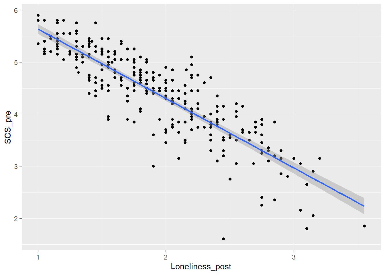

Did I do it right? yes no

Solution

The scatterplot is incorrect. Since we are predicting loneliness from social connectedness, the axes should be reversed.

In a correlation, the order of x and y does not matter, but in a regression, the predictor variable must be on the x-axis, and the outcome variable must be on the y-axis.

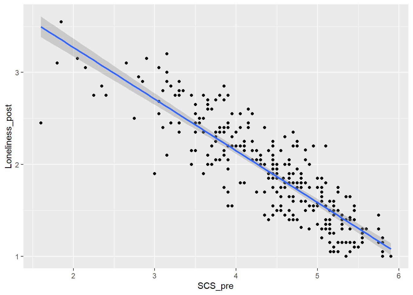
Here is the corrected scatterplot:

ggplot(dog_reg, aes(x = SCS_pre, y = Loneliness_post)) +
  geom_point() +
  geom_smooth(method = "lm")

`geom_smooth()` using formula = 'y ~ x'

Task 6: Model creating & Assumption checks

Let’s store our linear model as mod and then use the check_model() function from the performance package to check assumptions.

Remember, the structure of the linear model is:

lm(Outcome~Predictor, data)

Once the model is stored as mod, we can check its assumptions using check_model(mod).

Solution

## creating the linear model
mod <- lm(Loneliness_post~SCS_pre, data = dog_reg)

## checking model assumptions
check_model(mod)

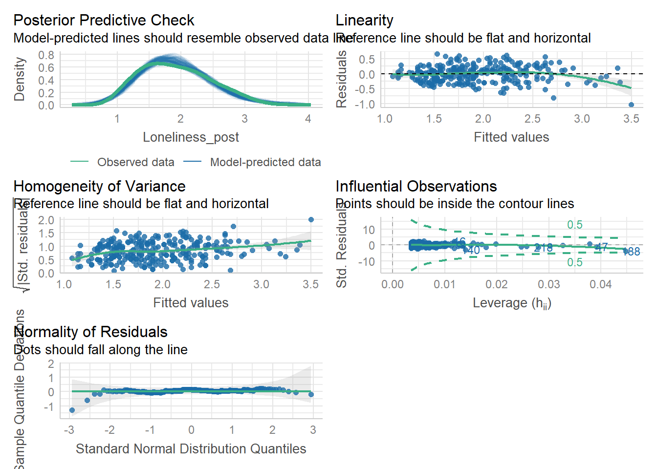
Assumptions 1-3 hold due to the study design, but let’s take a closer look at the following output:

• Linearity: The relationship appears to be non-linear linear.
• Normality: The residuals are approximately normally distributed not normally distributed.
• Homoscedasticity: There is homoscedasticity as there is no distinct pattern in the residuals heteroscedasticity as the residuals show a distinct pattern.

I don’t understand - can you explain more?

• Linearity: The reference line is mostly flat and horizontal. There’s a slight curve at the end, but when checking the scatterplot, it’s not a major concern.
• Normality: Looking pretty good. The dots fall onto the line, indicating the residuals are approximately normally distributed. A Q-Q plot would show the same outcome, but with the reference line diagonal instead of horizontal.
• Homoscedasticity (or Homogeneity of Variance): Yeah, the reference line could be a bit more horizontal, but there’s no clear funnel shape. The points appear to have a fairly random pattern, so we can consider the assumption met.

Task 7: Computing a Simple Regression & interpret the output

To compute the simple regression, we need to use the summary() on our linear model mod.

summary(mod)

How do you interpret the output?

• The estimate of the y-intercept for the model, rounded to two decimal places, is

• The relationship is positive negative

• The model indicated that Social Connectedness significantly predicts Loneliness post intervention. Social Connectedness does not significantly predicts Loneliness post intervention.

• How much the variance is explained by the model (rounded to two decimal places)? %.