
| RID | Loneliness_pre | Loneliness_post | Loneliness_diff |
|---|---|---|---|
| 1 | 2.25 | 1.70 | -0.55 |
| 2 | 1.90 | 1.60 | -0.30 |
| 3 | 2.25 | 2.25 | 0.00 |
| 4 | 1.75 | 2.05 | 0.30 |
| 5 | 2.85 | 2.70 | -0.15 |
2B Lab 1 Week 2
This is the pair coding activity related to Chapter 8.
Task 1: Open the R project for the lab
Task 2: Create a new .Rmd file
… and name it something useful. If you need help, have a look at Section 1.3.
Task 3: Load in the library and read in the data
The data should already be in your project folder. If you want a fresh copy, you can download the data again here: data_pair_coding.
We are using the packages rstatix, tidyverse, qqplotr, lsr today. Make sure to load rstatix in before tidyverse.
We also need to read in dog_data_clean_wide.csv. Again, I’ve named my data object dog_data_wide to shorten the name but feel free to use whatever object name sounds intuitive to you.
For the plot, we will need the data in long format. We can either read in dog_data_clean_long.csv to take a shortcut, or wrangle the data from dog_data_wide. I’ve taken the shortcut and named my data object dog_data_long.
Task 4: Tidy data for a paired t-test
Not much tidying to do for today.
Pick a variable of interest and select the pre- and post-scores, and calculate the difference score. Store them in a separate data object with a meaningful name.
I will use Loneliness as an example and call my data object dog_lonely. Regardless of your chosen variable, your data object should look like/ similar to the table below.
In dog_data_long, we want to turn Stage into a factor so we can re-order the labels (i.e., “pre” before “post”).
Task 5: Compute descriptives
We want to determine the mean and sd of:
- the pre-scores
- the post-scores, and
- the difference scores
Store them in a data object called descriptives.
Task 6: Check assumptions
Assumption 1: Continuous DV
Is the dependent variable (DV) continuous? Answer:Assumption 2: Data are independent
Each pair of values in the dataset has to be independent, meaning each pair of values needs to be from a separate participant. Answer:
Assumption 3: Normality
Looking at the violin-boxplots below, do you think the assumption of normality holds?
Note
The axis label of Plot 2 turned out to be quite long here. I’ve used the escape character \n to break it up across 2 lines.
## Plot 1
ggplot(dog_data_long, aes(x = Stage, y = Loneliness, fill = Stage)) +
  geom_violin(alpha = 0.5) +
  geom_boxplot(width = 0.4, alpha = 0.8) +
  scale_fill_viridis_d(guide = "none") +
  theme_classic() +
  labs(x = "Time point", y = "mean Loneliness Scores")

## Plot 2
ggplot(dog_lonely, aes(x = "", y = Loneliness_diff)) +
  geom_violin(fill = "#21908C", alpha = 0.5) +
  geom_boxplot(fill = "#21908C", width = 0.4) +
  theme_classic() +
  labs(x = "",
       y = "Difference in mean Loneliness scores \nbetween pre- and post- intervention") # \n forces a manual line break in the axis label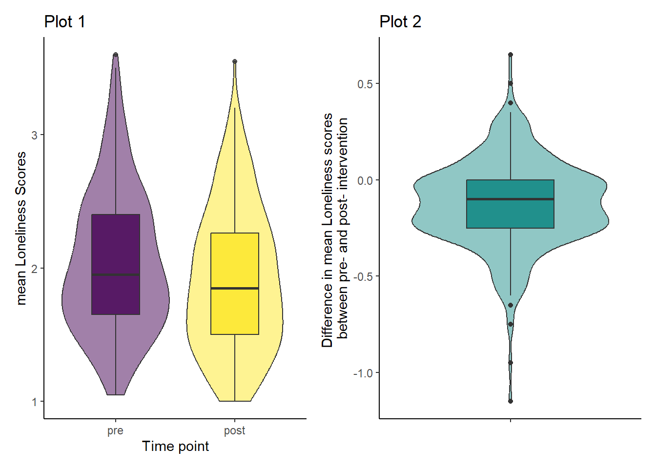
Answer:
Conclusion from assumption tests
With all assumptions tested, which statistical test would you recommend for this analysis?
Answer:Task 7: Computing a paired-sample t-test with effect size & interpret the output
- Step 1: Compute the paired-sample t-test. The structure of the function is as follows:
- Step 2: Calculate an effect size
Calculate Cohen’s D. The structure of the function is as follows:
- Step 3: Interpreting the output
Below are the outputs for the descriptive statistics (table), paired-samples t-test (main output), and Cohen’s D (last line starting with [1]). Based on these, write up the results in APA style and provide an interpretation.
| mean_pre | sd_pre | mean_post | sd_post | diff | sd_diff |
|---|---|---|---|---|---|
| 2.040187 | 0.5304488 | 1.914298 | 0.5344914 | -0.1258895 | 0.2290269 |
    Paired t-test

data:  dog_lonely$Loneliness_pre and dog_lonely$Loneliness_post
t = 9.2632, df = 283, p-value < 2.2e-16
alternative hypothesis: true mean difference is not equal to 0
95 percent confidence interval:
 0.09913876 0.15264034
sample estimates:
mean difference
      0.1258895
[1] 0.5496716We hypothesised that there would be a significant difference between Loneliness measured before (M = , SD = ) and after (M = , SD = ) the dog intervention. On average, participants felt less lonely after the intervention (Mdiff = , SDdiff = ). Using a paired-samples t-test, the effect was found to be and of a magnitude, t() = , p , d = . We therefore .