
2A Lab 8 Week 10
This is the pair coding activity related to Chapter 7.
Task 1: Open the R project for the lab
Task 2: Create a new .Rmd file
… and name it something useful. If you need help, have a look at Section 1.3.
Task 3: Load in the library and read in the data
The data should already be in your project folder. If you want a fresh copy, you can download the data again here: data_pair_coding.
We are using the packages tidyverse, car, and lsr today, and the data file we need to read in is dog_data_clean_wide.csv. I’ve named my data object dog_data_wide to shorten the name but feel free to use whatever object name sounds intuitive to you.
If you have not worked through chapter 7 yet, you may need to install a few packages first before you can load them into the library, for example, if car is missing, run install.packages("car") in your CONSOLE.
Task 4: Tidy data for a two-sample t-test
For today’s task, we want to analyse how students’ psychological well-being scores differed at the post_intervention time point. Specifically, we will compare the scores of students who directly interacted with the dogs (Group direct)to those who only talked to the dog handlers (Group control).
To achieve that, we need to select all relevant columns from dog_data_wide, and narrow down the dataframe to only include students assigned either to the direct or the control groups.
Step 1: Select all relevant columns from
dog_data_wide. For the task at hand, those would be the participant IDRID,GroupAssignment, andFlourishing_post. Store this data in an object calleddog_independent.Step 2: Narrow down
dog_independentto only includeGroupAssignmentgroupsdirector thecontrol.Step 3: Convert
GroupAssignmentinto a factor.
Task 5: Compute descriptives
Calculate the sample size (n), the mean, and the standard deviation of the psychological well-being score for both groups. Save the output in an object called dog_independent_descriptives. The resulting dataframe should look like this:
| GroupAssignment | n | mean_Flourishing | sd_Flourishing |
|---|---|---|---|
| Control | 94 | 5.718085 | 0.7709738 |
| Direct | 95 | 5.776316 | 0.8638912 |
Task 6: Check assumptions
Assumption 1: Continuous DV
Is the dependent variable (DV) continuous? Answer:Assumption 2: Data are independent
Each observation in the dataset has to be independent, meaning the value of one observation does not affect the value of any other. Answer:
Assumption 3: Homoscedasticity (homogeneity of variance)
I’ve computed Levene’s test below. How do you interpret the output?
| Df | F value | Pr(>F) | |
|---|---|---|---|
| group | 1 | 0.7111707 | 0.4001329 |
| 187 | NA | NA |
Assumption 4: DV should be approximately normally distributed
Looking at the violin-boxplot below, are both groups normally distributed?
ggplot(dog_independent, aes(x = GroupAssignment, y = Flourishing_post, fill = GroupAssignment)) +
  geom_violin(alpha = 0.4) +
  geom_boxplot(width = 0.3, alpha = 0.8) +
  scale_fill_viridis_d(option = "cividis", guide = "none") +
  theme_classic() +
  labs(x = "Group", y = "Psychological well-being (post-intervention)")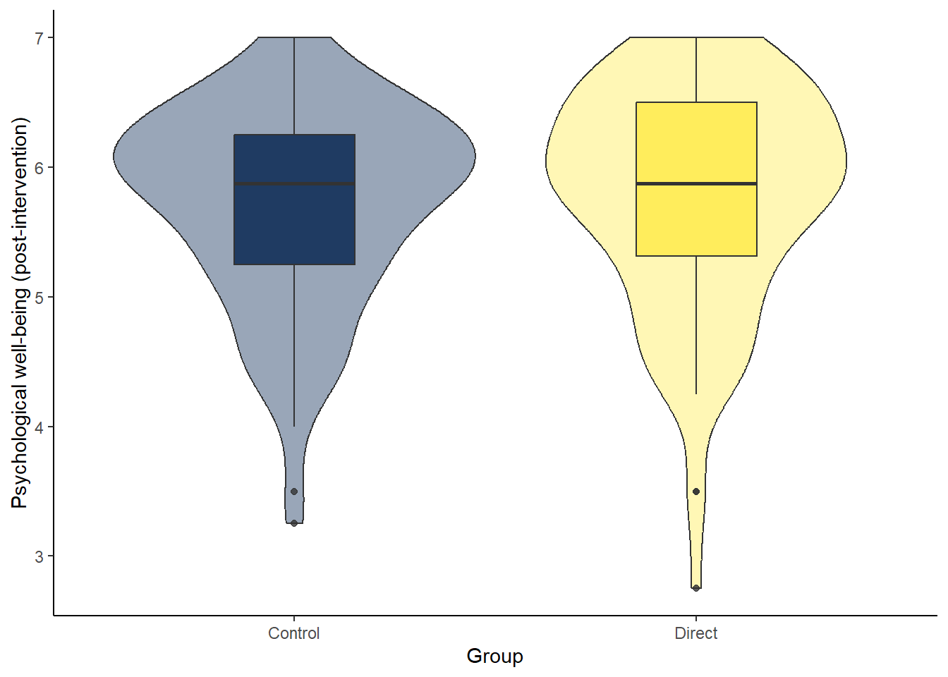
Answer:
Conclusion from assumption tests
With all assumptions tested, which statistical test would you recommend for this analysis?
Answer:Task 7: Computing a two-sample t-test with effect size & interpret the output
- Step 1: Compute the Welch two-sample t-test. The structure of the function is as follows:
- Step 2: Calculate an effect size
Calculate Cohen’s D. The structure of the function is as follows:
- Step 3: Interpreting the output
Below are the outputs for the descriptive statistics (table), Welch t-test (main output), and Cohen’s D (last line starting with [1]). Based on these, write up the results in APA style and provide an interpretation.
| GroupAssignment | n | mean_Flourishing | sd_Flourishing |
|---|---|---|---|
| Control | 94 | 5.718085 | 0.7709738 |
| Direct | 95 | 5.776316 | 0.8638912 |
    Welch Two Sample t-test

data:  Flourishing_post by GroupAssignment
t = -0.48902, df = 185.05, p-value = 0.6254
alternative hypothesis: true difference in means between group Control and group Direct is not equal to 0
95 percent confidence interval:
 -0.2931533  0.1766920
sample estimates:
mean in group Control  mean in group Direct
             5.718085              5.776316
[1] 0.0711213The Welch two-sample t-test revealed that there is in psychological well-being scores between direct (N = , M = , SD = ) and control group (N = , M = , SD = ), t() = , p = , d = . The strength of the association between the variables is considered . We therefore .