Chapter 2 Introduction to Data

Intended Learning Outcomes

1. understand basic data types
2. create and store vectors
3. convert data types into one another
4. create a data table from scratch
5. import and store data

This lesson is led by Gaby Mahrholz.

2.1 Pre-Steps

Before we begin, we need to do some house-keeping.

2.1.1 Downloading materials

First, we need to download the materials we are working with today. You can find them on moodle. It’s a zip folder that contains an Rmd file called L2_stub and a data file in .csv format for later. L2_stub has all the code chunks listed for today’s lesson. You are more than welcome to add notes and comments to the Rmd (white chunks), however there is no need to copy any code.

2.1.2 Unzipping the zip folder

The folder we have downloaded is a zip folder. R cannot handle zip folders very well, so the folder needs to be unzipped. Right-mouseclick on the zipped folder, then choose Extract All....

Copy and paste/ move the folder to your M drive (or somewhere that makes sense to you - and where you can find it again - if you are using your own computer).

Check the unzipped folder contains the L2_stub.Rmd and a data file called MM_data.csv.

2.1.3 Setting the working directory

It is always good practice to set your working directory to the folder you are working with. This can be done in 2 ways:

1. In the menu, go to Session > Set Working Directory > Choose Directory (Ctrl + Shift + H also works as key short cut in a Windows environment). Then select the folder containing the data file and click ‘open’. You might not see any files in the folder you are selecting - that is fine.

2. In the Files pane, you could navigate to today’s folder, and once there click on More > Set As Working Directory.

Whichever way you prefer is fine. The files L2_stub and MM_data.csv should now be visible in the Files pane.

2.1.4 Load tidyverse into the library

We will be using a few functions today that are part of the tidyverse package compilation. Let’s load tidyverse in the library now, so we do not have to worry about it later on.

library(tidyverse)

Yay, with that out of the way, we can begin Lesson 2.

2.2 Basic data types

There are plenty data types, however for our purposes we will be focussing on:

data type	description	example
character	text string	"hello World!", "35.2", 'TRUE'
double	double precision floating point numbers	.033, -2.5
integer	positive & negative whole numbers	0L, 1L, 365L
logical	Boolean operator with only two possible values	TRUE, FALSE

2.2.1 Character

You can store any text as a value in your local environment. You can either use single or double inverted commas.

my_quote <- 'R is Fun to learn!'
cat(my_quote) # cat() prints the value stored in my_quote

If you want to use a direct quote, you need to include a backslash before each inverted comma.

direct_quote <- "My friend said \"R is Fun to learn\", and we all agreed."
cat(direct_quote)

## My friend said "R is Fun to learn", and we all agreed.

You can check the data type using the typeof() function. If you want to know which class they belong to, you can use the class() function.

2.2.2 Numeric

double and integer are both class numeric. Double is a number with decimal places whereas integer is a number that’s a full number. Any number will be stored as a double unless you specify integer by adding an L as a suffix.

Example:

typeof(359.1)

## [1] "double"

typeof(5)

## [1] "double"

typeof(45L)

## [1] "integer"

2.2.3 Logical

A logical vector is a vector that only contains TRUE and FALSE values. You can use that type of data to compare (or relate) 2 pieces of information. We have several comparison (or relational) operators in R. A few of them are:

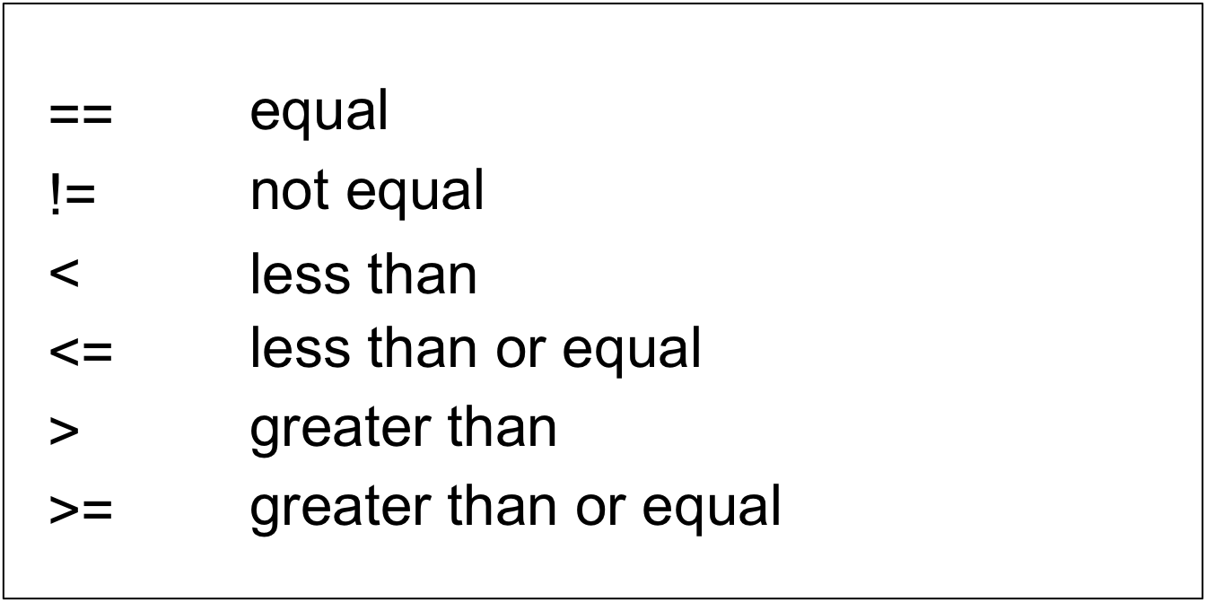
More information on logical comparison operators can be found on https://bookdown.org/ndphillips/YaRrr/logical-indexing.html (from which the above image was modified).

You could compare if two values are equal…

100 == 100

## [1] TRUE

… or if they are not equal.

100 != 100

## [1] FALSE

We can test if one value is smaller or equal than the other…

5 <= 9-4

## [1] TRUE

… or if one value is larger than another.

101 > 111

## [1] FALSE

Note that it works with character strings as well. (Not really important for this class though)

# "a" == "a" would be TRUE as both side of the comparison contain the same information.
"a" == "a"

## [1] TRUE

# "a" <= "b" would be TRUE as a comes before b in the alphabet (i.e. 1st letter vs 2nd letter)
"a" <= "b"

## [1] TRUE

# "abc" > "a" would be TRUE as there are more values on the left than on the right
"abc" > "a"

## [1] TRUE

Question Time

Run the following examples in your Console and select from the drop down menu what data type they belong to:

• class(1): character double integer logical Error message
• class(1L): character double integer logical Error message
• class(1.0): character double integer logical Error message
• class(“1”): character double integer logical Error message
• class(1L == 2L): character double integer logical Error message
• class(1L <= 2L): character double integer logical Error message
• class(1L <= 2L, “1”): character double integer logical Error message

Any number will be stored as a double unless you specify integer by adding an L as a suffix.

2.3 Vectors

Vectors are one of the very simple data structure in R. You could define them as “a single entity consisting of a collection of things”.

2.3.1 Creating vectors

If you want to combine more than one element into one vector, you can do that by using the c() function. c stands for combine or as my colleague once said, it’s hugging multiple elements together. All elements in the vector have to be of the same data type.

Examples:

This is a vector of datatype double.

c(1, 2.5, 4.7)

## [1] 1.0 2.5 4.7

typeof(c(1, 2.5, 4.7))

## [1] "double"

This is a vector of datatype integer. Adding the L makes it an integer, but see that in the printout the L is actually omitted.

c(0L, 1L, 2L, 365L)

## [1]   0   1   2 365

typeof(c(0L, 1L, 2L, 365L))

## [1] "integer"

This is a vector of datatype character.

c("hello", "student")

## [1] "hello"   "student"

typeof(c("hello", "student"))

## [1] "character"

This is a vector of datatype logic.

c(TRUE, FALSE)

## [1]  TRUE FALSE

typeof(c(TRUE, FALSE))

## [1] "logical"

We have seen what vectors look like. If you want to store these vectors in your global environment, all you need is the assignment operator <- and a meaingful name for “the thing” you want to store. Here the first example reads like: “Take a vector of 3 elements (namely 1, 2.5, 4.7) and store it in your Global Environment under the name vec_double.” You can then use the name you assigned to the vector within the typeof() function, rather than the vector itself.

vec_double <- c(1, 2.5, 4.7)
typeof(vec_double)

## [1] "double"

vec_integer <- c(0L, 1L, 2L, 365L)
typeof(vec_integer)

## [1] "integer"

vec_character <- c("hello", "student")
typeof(vec_character)

## [1] "character"

vec_logic <- c(TRUE, FALSE)
typeof(vec_logic)

## [1] "logical"

Funnily enough, a vector i <- c(1,3,4,6) would be stored as a double. However, when coded as i <- 1:10 would be stored as an integer.

Don’t believe it? Try it out in your Console!

Question Time

Your turn

• Create a vector of your 3 favourite movies and call it favourite_movies. What type of data are we expecting?

• Pick a couple of your family members or friends and create a vector years_birth that lists their year of birth. How many elements does the vector have, and what type of data are we expecting?

• Create a vector that holds all the letters of the alphabet and call it alph.

• Create a vector with 3 elements of your name, age, and the country you are from. Store this vector under the name this_is_me. What type of data are we expecting?

# Gaby's solution:
favourite_movies <- c("Red", "Cloud Atlas", "Hot Fuzz") # character
years_birth <- c(1953, 1975) # double
alph <- letters # muahahahaaaa! & character
this_is_me <- c("Gaby", 38, "Germany") # character

More detailed explanations:

R has Built-in Constants:

• letters: the 26 lower-case letters of the Roman alphabet;
  
• LETTERS: the 26 UPPER-case letters of the Roman alphabet;
  
• month.abb: the three-letter abbreviations for the English month names;
  
• month.name: the English names for the months of the year;
  
• pi: the ratio of the circumference of a circle to its diameter

Of course, the task could have been solved typing alph <- c(“a”, “b”, “c”, “d”, “e”, “f”, “g”, “h”, “i”, “j”, “k”, “l”, “m”, “n”, “o”, “p”, “q”, “r”, “s”, “t”, “u”, “v”, “w”, “x”, “y”, “z”)

this_is_me would be stored as a character vector despite having text as well as numeric elements. Remember how we said earlier that all elements have to be of the same data type? After the next section, you will understand why they are stored as a character and not as a numeric vector.

2.3.2 Converting vectors into different data types of vectors aka funky things we can do

We can also reassign data types to our vectors we have just created. For example if we wanted to turn our var_double from double to character, we would code

vec_double_as_char <- as.character(vec_double)
typeof(vec_double_as_char)

## [1] "character"

In your Global Environment, you can now see that the vector vec_double has 3 numeric elements (abbreviated num), whereas vec_double_as_char has 3 character elements (abbreviated chr). Also note that the numbers 1.2, 2.5, and 4.7 have now quotation marks around them.

Likewise, if we wanted to turn our integer vector vec_integer into data type double, we would use

vec_integer_as_double <- as.double(vec_integer)
typeof(vec_integer_as_double)

## [1] "double"

In your Global Environment, see how vec_integer has int assigned to it, whereas vec_integer_as_double is now listed as num. The typeof function revealed that the 4 elements of vec_integer_as_double are now stored as data type double.

However, trying to turn a character vector into an integer or a double would fail.

vec_char_as_int <- as.integer(vec_character) # same outcome if we tried as.double

## Warning: NAs introduced by coercion

typeof(vec_char_as_int)

## [1] "integer"

R would still compute “something” but it would be accompanied by the above warning message. As you can see in your Global Environment, vec_char_as_int does indeed exist as a numeric vector with 2 elements, but NA tells us they are classified as missing values.

A logical vector can be converted into all other basic data types.

vec_logic_as_int <- as.integer(vec_logic)
vec_logic_as_int

## [1] 1 0

TRUE and FALSE will be coded as 1 and 0 respectively when converting a logical into a numeric vector (integer or double). When converting a logical into a characters, it will just read as "TRUE" and "FALSE".

vec_logic_as_char <- as.character(vec_logic)
vec_logic_as_char

## [1] "TRUE"  "FALSE"

Question Time

Remember the vector this_is_me? Can you explain now why it was stored as character?

this_is_me would be stored as a character vector because this is the best way to retain all information. If this were to be stored as a numeric vector, the name and home country could only be coded as missing values NA. So rather than trying to turn everything into a number (which is not possible/ does not retain meaningful information), R turns the number into character (which is possible).

With this in mind, what data type would the vector be stored as if you combined the following elements?

1. logical and double - i.e. c(TRUE, 45)
2. character and logical - i.e. c(“Sarah”, “Marc”, FALSE)
3. integer and logical - i.e. c(1:3, TRUE)
4. logical, double, and integer - i.e. c(FALSE, 99.5, 3L)

1. double
2. character
3. integer
4. double

2.3.3 Adding elements to existing vectors

Let’s start with a vector called friends that has three names in it.

friends <- c("Gaby", "Wil", "Greta")
friends

## [1] "Gaby"  "Wil"   "Greta"

We can now add more friends to our little group of friends by adding them either at the end, or the beginning of the vector. friends will now have four, and five values respectively, since we are “overwriting” our existing vector with the new one of the same name.

friends <- c(friends, "Kate")
friends

## [1] "Gaby"  "Wil"   "Greta" "Kate"

friends <- c("Rebecca", friends)
friends

## [1] "Rebecca" "Gaby"    "Wil"     "Greta"   "Kate"

Vectors also support missing data. If we wanted to add “another friend” whose name we do not know yet, we can just simply add NA to friends.

friends <- c(friends, NA)
friends

## [1] "Rebecca" "Gaby"    "Wil"     "Greta"   "Kate"    NA

The vector friends would still be a character vector. Missing values do not alter the original data type. However, if you look in the Global Environment, you can see that the number of elements stored in friends increased from 5 to 6. To determine the number of elements in a vector in R (rather than eye sight), you can also use a function called length().

typeof(friends)

## [1] "character"

length(friends)

## [1] 6

Well, now we decided that 5 friends in our little group of friends is sufficient, and we did not want anyone else to join, we could remove the “placeholder friend NA” by coding

friends <- friends[1:5]
friends

## [1] "Rebecca" "Gaby"    "Wil"     "Greta"   "Kate"

You can see that the length of the vector friends is now back to 5 again.

1:5 uses the colon operator: which is read as in “access the vector elements 1, 5, and everything in between”. An alternative way of writing out the above without using a colon operator would be friends[c(1,2,3,4,5)]. Notice that you need the c() function again.

Just as easily, we can create vectors for numeric sequences. The function seq() is a neat way of doing this, or you can use the colon operator: again. Just with the elements in the vector above, the same logic applies here. For example 1:10 means, you want to list number 1, number 10, and all numbers in between.

sequence1 <- 1:10
sequence1

##  [1]  1  2  3  4  5  6  7  8  9 10

sequence2 <- seq(10)
sequence2

##  [1]  1  2  3  4  5  6  7  8  9 10

# compare whether sequence1 and sequence2 are of the same data type
typeof(sequence1) == typeof(sequence2)

## [1] TRUE

# compare whether elements of sequence1 are the same as the elements in sequence2 
sequence1 == sequence2

##  [1] TRUE TRUE TRUE TRUE TRUE TRUE TRUE TRUE TRUE TRUE

Question Time

• What data type is sequence1? character double integer logical
• What data type is sequence2? character double integer logical
• If we were to store the output of sequence1 == sequence2 in a vector, what data type would the vector be? character double integer logical

2.4 Tibble - the new way of creating a dataframe

2.4.1 What the heck is a tibble? Do you mean table?

First of all, tibble is not a spelling error; it’s the way r refers to its newest form of data table or dataframe. You can create a dataframe either by using the tibble() function or a function called data.frame(). tibble() is part of the package tidyverse whereas data.frame can be found in base R and does not need an additional package read into the library. Tibbles are slightly different to dataframes in that

• they have better print properties (Dataframes print ALL data when you call the data whereas tibbles only print the first 10 rows of data)
• character vectors are not coerced into factors (which you will be thankful for later on in your programming life)
• column names are not modified (for example if you wanted to make a column called Female Voices you could just do that. tibble keeps it as Female Voices with a space between the two words, whereas the data.table function would change it to Female.Voices)

If you want to read more about the differences between dataframes and tibbles (and appreciate the advantages of tibbles), have a look on https://cran.r-project.org/web/packages/tibble/vignettes/tibble.html.

2.4.2 How to make a tibble from scratch

Now that you have learnt how to create vectors, we can try and combine them into a tibble. The easiest way is to use the tibble() function. Let’s say we want to create a tibble that is called tibble_year with 4 columns:

• The first column month lists all months of the year
• The second column abb_month gives us the three-letter abbreviation of each year.
• The third column month_num tells which number of the year is which month (e.g. January would be the first month of the year; December would be number 12).
• The fourth column season would tell us in which season the month is (Northern hemisphere).

Remember the Built-in Constants we were talking about earlier?

# Remember to load tidyverse into your script at least once (usually at the beginning)
library(tidyverse)

tibble_year <- tibble(month = month.name,
                      abb_month = month.abb,
                      month_num = 1:12,
                      season = c(rep("Winter", 2), rep("Spring", 3), rep("Summer", 3), rep("Autumn", 3), "Winter"))

tibble_year

## # A tibble: 12 x 4
##    month     abb_month month_num season
##    <chr>     <chr>         <int> <chr> 
##  1 January   Jan               1 Winter
##  2 February  Feb               2 Winter
##  3 March     Mar               3 Spring
##  4 April     Apr               4 Spring
##  5 May       May               5 Spring
##  6 June      Jun               6 Summer
##  7 July      Jul               7 Summer
##  8 August    Aug               8 Summer
##  9 September Sep               9 Autumn
## 10 October   Oct              10 Autumn
## 11 November  Nov              11 Autumn
## 12 December  Dec              12 Winter

The generic structure of each of these columns we are creating is column header name = values to fill in the rows.

Here, we used the built-in replication function rep() to build the column season which is a more time-efficient approach than typing out 4 seasons 3 times. Of course, we could have written season = c(“Winter”, “Winter”, “Spring”, “Spring”, “Spring”, “Summer”, “Summer”, “Summer”, “Autumn”, “Autumn”, “Autumn”, “Winter”) instead.

We can now use the function glimpse() to see which data types our columns are. This is a very handy function to keep in mind for later!

glimpse(tibble_year)

## Observations: 12
## Variables: 4
## $ month     <chr> "January", "February", "March", "April", "May", "June", "...
## $ abb_month <chr> "Jan", "Feb", "Mar", "Apr", "May", "Jun", "Jul", "Aug", "...
## $ month_num <int> 1, 2, 3, 4, 5, 6, 7, 8, 9, 10, 11, 12
## $ season    <chr> "Winter", "Winter", "Spring", "Spring", "Spring", "Summer...

glimpse() tells us that our tibble has one column that is an integer, and three columns that are character strings. If we wanted to influence which datatype the columns (something that is not automatically assigned), we can do that by using the functions as.double(), as.character(), as.integer(), etc. we have seen earlier when we were talking about vectors. For example, if we wanted to modify the integer column as a double, we would type

tibble_year2 <- tibble(month = month.name,
                       abb_month = month.abb,
                       month_num = as.double(1:12),
                       season = c(rep("Winter", 2), rep("Spring", 3), rep("Summer", 3), rep("Autumn", 3), "Winter"))

If you click on the name of the dataset in your Global Environment to view your dataframe, you would see no actual difference between tibble_year and tibble_year2. However, glimpse() would tell you.

If I were a mean person, and had recoded month_num = as.character(1:12) instead, you would not see it when you visually inspect the data. What would the consequences be?

Question Time

Your turn

Make a tibble called mydata with 5 columns and 10 rows:

• column 1 is called PP_ID and contains participant numbers 1 to 10. Make sure this data type is integer.
• column 2 is called PP_Age and and contains the age of the participant. Make sure this data type is double.
• column 3 is called PP_Sex and contains the sex of the participant. Even PP_IDs are male, odd PP_IDs are female participants.
• column 4 is called PP_Country and contains the country participants were born in. Surprise, surprise - they were all born in Scotland!!!
• column 5 is called PP_Consent and is an overview whether participants have given their consent to participate in an experiment (TRUE) or not (FALSE). Participants 1-9 have given their consent, participant 10 has not.

# Gaby's solution:
mydata <- tibble(PP_ID = 1:10,
                 PP_Age = c(22, 21, 24, 36, 33, 25, 21, 31, 28, 35),
                 PP_Sex = rep(c("Female", "Male"), 5),
                 PP_Country = "Scotland",
                 PP_Consent = c(rep(TRUE, 9), FALSE))

But there are plenty of other ways how this could have been done. For example:

• PP_ID = seq(10)
  
• PP_ID = as.integer(c(1, 2, 3, 4, 5, 6, 7, 8, 9, 10))
  
• PP_Age = as.double(22:31)
  
• PP_Sex = c(“Female”, “Male”, “Female”, “Male”, “Female”, “Male”, “Female”, “Male”, “Female”, “Male”)
  
• PP_Country = rep(“Scotland”, 10)
  
• PP_Consent = c(TRUE, TRUE, TRUE, TRUE, TRUE, TRUE, TRUE, TRUE, TRUE, FALSE)

2.5 Reading in data

2.5.1 from pre-existing databases

R comes with pre-installed datasets available for you to use and practice your skills on. If you want have an overview over all databases available type data() into your Console.

One of those datasets is called “Motor Trend Car Road Tests” or in short mtcars. If you type mtcars into your Console, you can see what the dataset looks like.

mtcars

##                      mpg cyl  disp  hp drat    wt  qsec vs am gear carb
## Mazda RX4           21.0   6 160.0 110 3.90 2.620 16.46  0  1    4    4
## Mazda RX4 Wag       21.0   6 160.0 110 3.90 2.875 17.02  0  1    4    4
## Datsun 710          22.8   4 108.0  93 3.85 2.320 18.61  1  1    4    1
## Hornet 4 Drive      21.4   6 258.0 110 3.08 3.215 19.44  1  0    3    1
## Hornet Sportabout   18.7   8 360.0 175 3.15 3.440 17.02  0  0    3    2
## Valiant             18.1   6 225.0 105 2.76 3.460 20.22  1  0    3    1
## Duster 360          14.3   8 360.0 245 3.21 3.570 15.84  0  0    3    4
## Merc 240D           24.4   4 146.7  62 3.69 3.190 20.00  1  0    4    2
## Merc 230            22.8   4 140.8  95 3.92 3.150 22.90  1  0    4    2
## Merc 280            19.2   6 167.6 123 3.92 3.440 18.30  1  0    4    4
## Merc 280C           17.8   6 167.6 123 3.92 3.440 18.90  1  0    4    4
## Merc 450SE          16.4   8 275.8 180 3.07 4.070 17.40  0  0    3    3
## Merc 450SL          17.3   8 275.8 180 3.07 3.730 17.60  0  0    3    3
## Merc 450SLC         15.2   8 275.8 180 3.07 3.780 18.00  0  0    3    3
## Cadillac Fleetwood  10.4   8 472.0 205 2.93 5.250 17.98  0  0    3    4
## Lincoln Continental 10.4   8 460.0 215 3.00 5.424 17.82  0  0    3    4
## Chrysler Imperial   14.7   8 440.0 230 3.23 5.345 17.42  0  0    3    4
## Fiat 128            32.4   4  78.7  66 4.08 2.200 19.47  1  1    4    1
## Honda Civic         30.4   4  75.7  52 4.93 1.615 18.52  1  1    4    2
## Toyota Corolla      33.9   4  71.1  65 4.22 1.835 19.90  1  1    4    1
## Toyota Corona       21.5   4 120.1  97 3.70 2.465 20.01  1  0    3    1
## Dodge Challenger    15.5   8 318.0 150 2.76 3.520 16.87  0  0    3    2
## AMC Javelin         15.2   8 304.0 150 3.15 3.435 17.30  0  0    3    2
## Camaro Z28          13.3   8 350.0 245 3.73 3.840 15.41  0  0    3    4
## Pontiac Firebird    19.2   8 400.0 175 3.08 3.845 17.05  0  0    3    2
## Fiat X1-9           27.3   4  79.0  66 4.08 1.935 18.90  1  1    4    1
## Porsche 914-2       26.0   4 120.3  91 4.43 2.140 16.70  0  1    5    2
## Lotus Europa        30.4   4  95.1 113 3.77 1.513 16.90  1  1    5    2
## Ford Pantera L      15.8   8 351.0 264 4.22 3.170 14.50  0  1    5    4
## Ferrari Dino        19.7   6 145.0 175 3.62 2.770 15.50  0  1    5    6
## Maserati Bora       15.0   8 301.0 335 3.54 3.570 14.60  0  1    5    8
## Volvo 142E          21.4   4 121.0 109 4.11 2.780 18.60  1  1    4    2

You can look up what all the column headers mean by typing ?mtcars into your Console, or using the help tab to search for mtcars.

mtcars is a dataframe rather than a tibble. How do we know that?

When we called mtcars it printed the whole dataframe rather than just the first 10 rows.

However, we have seen what the data in mtcars looks now, but we would be able to work with it better if put it into our Global Environment. Let’s save mtcars as a dataframe called data_mtcars, and look at the first few rows which can be achieved using the head() function.

data_mtcars <- mtcars # read in as a dataframe
head(data_mtcars)

##                    mpg cyl disp  hp drat    wt  qsec vs am gear carb
## Mazda RX4         21.0   6  160 110 3.90 2.620 16.46  0  1    4    4
## Mazda RX4 Wag     21.0   6  160 110 3.90 2.875 17.02  0  1    4    4
## Datsun 710        22.8   4  108  93 3.85 2.320 18.61  1  1    4    1
## Hornet 4 Drive    21.4   6  258 110 3.08 3.215 19.44  1  0    3    1
## Hornet Sportabout 18.7   8  360 175 3.15 3.440 17.02  0  0    3    2
## Valiant           18.1   6  225 105 2.76 3.460 20.22  1  0    3    1

Notice that we do not have a column header for the type of car. The reason is that the type of car is actually the name of the rows, rather than a column itself. As you can see in your Global Environment, df_mtcars has 32 observations, and 11 variables - car type is not one of them.

Adding the rownames as a separate column would be rather tricky at this stage in the course (but you could try and do it after lecture 5).

Another interesting dataset is called starwars. It can be found in the package dplyr which is part of tidyverse. So, as long as you have tidyverse loaded into your library, starwars should be available to you.

library(tidyverse) # if you have already done this in your Rmd, this step is superfluous
starwars

## # A tibble: 87 x 13
##    name  height  mass hair_color skin_color eye_color birth_year gender
##    <chr>  <int> <dbl> <chr>      <chr>      <chr>          <dbl> <chr> 
##  1 Luke~    172    77 blond      fair       blue            19   male  
##  2 C-3PO    167    75 <NA>       gold       yellow         112   <NA>  
##  3 R2-D2     96    32 <NA>       white, bl~ red             33   <NA>  
##  4 Dart~    202   136 none       white      yellow          41.9 male  
##  5 Leia~    150    49 brown      light      brown           19   female
##  6 Owen~    178   120 brown, gr~ light      blue            52   male  
##  7 Beru~    165    75 brown      light      blue            47   female
##  8 R5-D4     97    32 <NA>       white, red red             NA   <NA>  
##  9 Bigg~    183    84 black      light      brown           24   male  
## 10 Obi-~    182    77 auburn, w~ fair       blue-gray       57   male  
## # ... with 77 more rows, and 5 more variables: homeworld <chr>, species <chr>,
## #   films <list>, vehicles <list>, starships <list>

In comparison to mtcars, starwars is already a tibble (which you can see in the first line of the printout). It gives you the number of observations (87) and variables (13), the column headers, the data type of each column, and the first 10 rows of data. Again, it would be neater to work with the data if we saved the data tibble to our Global Environment. Let’s do that and call it data_SW.

data_SW <- starwars

Again, you could use the very handy glimpse() function to see what data types the columns are.

glimpse(data_SW)

There are other built in datasets available, such as babynames. The babynames dataset is located in a package called babynames which needs to be installed first, and then loaded into the library before you can look at the data. Do you remember how we install packages and load them into the library?

install.packages(“babynames”)
library(babynames)

Remember that you only have to do the install.packages(“babynames”) once - before you want to use babynames for the very first time. Once you have installed it, you can use it whenever you feel like by just loading it into the library.

2.5.2 from existing data files

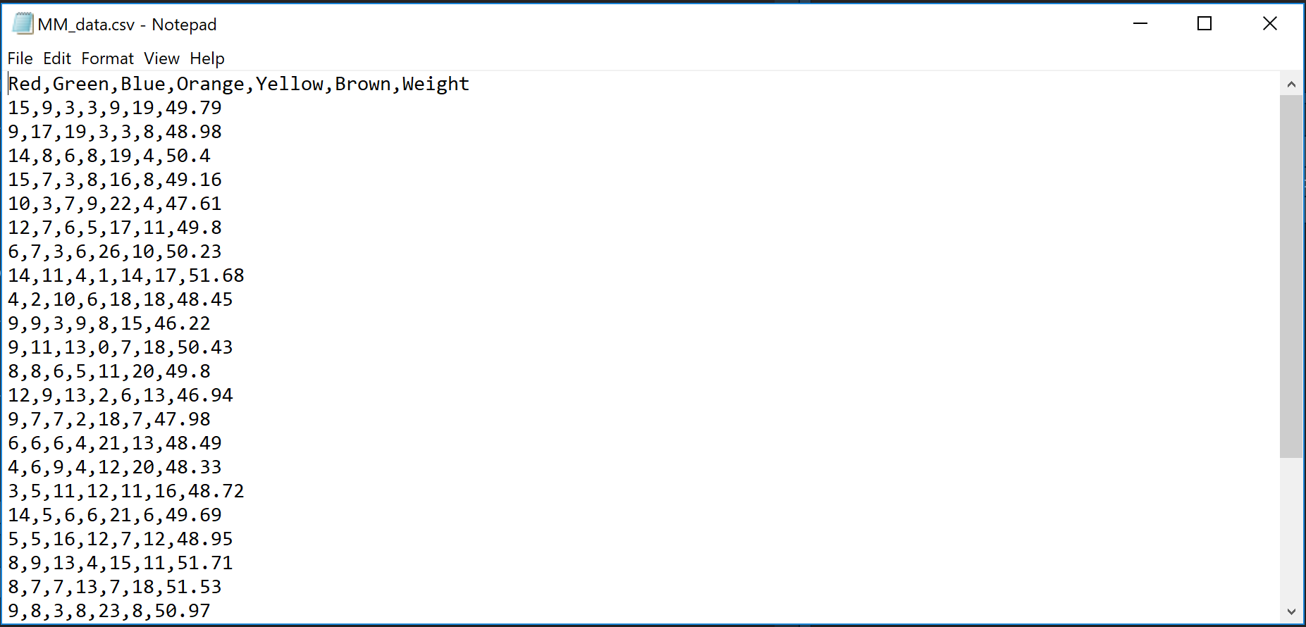
R is able to handle different types of data files. The most common one available is .csv. CSV stands for comma-separated values. Usually, a .csv file is opened with some sort of excel programme (like Microsoft Excel, LibreOffice, OpenOffice, Apple Numbers, etc.) which takes the comma separator as a mean to format everything into a nice and neat table. If you open your data in Notepad, you can actually see the structure of it.

There are other file types out there, apart from csv, like tsv (tab-separated values), excel, SAS, or SPSS. However, these would go beyond the scope of this class. All of our data will be in a .csv format.

Getting the data from the csv file into your Global Environment in R is by using a function called read_csv() from the package tidyverse. Since we did the house-keeping (i.e. loading in the package tidyverse into the library) at the very beginning, there is no need for us to do that again.

The data you just saw in the screenshot above are from M&Ms colours by bag (http://www.randomservices.org/random/data/index.html). The data table gives the color counts and net weight (in grams) for a sample of 30 bags of M&M’s. The advertised net weight is 47.9 grams.

MM_data <- read_csv("MM_data.csv")

## Parsed with column specification:
## cols(
##   Red = col_double(),
##   Green = col_double(),
##   Blue = col_double(),
##   Orange = col_double(),
##   Yellow = col_double(),
##   Brown = col_double(),
##   Weight = col_double()
## )

As you can see, R is giving you a bit of an output of what it has just done - parsed some columns. The data is stored as an object in your Global Environment now, and we could either call the data (by typing MM_data into the Console) or use glimpse() to have a look what the data actually looks like and what data types are in each column.

MM_data

## # A tibble: 30 x 7
##      Red Green  Blue Orange Yellow Brown Weight
##    <dbl> <dbl> <dbl>  <dbl>  <dbl> <dbl>  <dbl>
##  1    15     9     3      3      9    19   49.8
##  2     9    17    19      3      3     8   49.0
##  3    14     8     6      8     19     4   50.4
##  4    15     7     3      8     16     8   49.2
##  5    10     3     7      9     22     4   47.6
##  6    12     7     6      5     17    11   49.8
##  7     6     7     3      6     26    10   50.2
##  8    14    11     4      1     14    17   51.7
##  9     4     2    10      6     18    18   48.4
## 10     9     9     3      9      8    15   46.2
## # ... with 20 more rows

glimpse(MM_data)

## Observations: 30
## Variables: 7
## $ Red    <dbl> 15, 9, 14, 15, 10, 12, 6, 14, 4, 9, 9, 8, 12, 9, 6, 4, 3, 14...
## $ Green  <dbl> 9, 17, 8, 7, 3, 7, 7, 11, 2, 9, 11, 8, 9, 7, 6, 6, 5, 5, 5, ...
## $ Blue   <dbl> 3, 19, 6, 3, 7, 6, 3, 4, 10, 3, 13, 6, 13, 7, 6, 9, 11, 6, 1...
## $ Orange <dbl> 3, 3, 8, 8, 9, 5, 6, 1, 6, 9, 0, 5, 2, 2, 4, 4, 12, 6, 12, 4...
## $ Yellow <dbl> 9, 3, 19, 16, 22, 17, 26, 14, 18, 8, 7, 11, 6, 18, 21, 12, 1...
## $ Brown  <dbl> 19, 8, 4, 8, 4, 11, 10, 17, 18, 15, 18, 20, 13, 7, 13, 20, 1...
## $ Weight <dbl> 49.79, 48.98, 50.40, 49.16, 47.61, 49.80, 50.23, 51.68, 48.4...

You could also have used the function head() to show the first 6 rows of the dataframe or could have viewed the data by clicking manually on MM_data in the Global Environment.

Watch out, though!!! head() can be a bit misleading in that it creates a new tibble and the output reads # A tibble: 6 x 7. This does not mean that our MM_data only has 6 rows of observations!!!

Viewing the data opens the data in a new tab in the Source pane but it does not show you the data types of the columns. You could, however, click on the wee blue arrow next to the data name.

Now that we have inspected the data, what does it actually tell us?

Question Time

How many rows (or observations) does MM_data have?
How many columns (or variables) does MM_data have?
What data type are all of the columns? character double integer logical

Always use read_csv() from the tidyverse package for reading in the data. There is a similar function called read.csv() from base R - DO NOT USE read.csv(). These two functions have differences in assigning datatypes to the columns and read_csv() does a better job. This applies to the homework task as well. You will not receive marks if you are using the wrong function. So double check before submitting!!!

2.6 Last point for today

Restart R and clear your workspace. Knit your L2_stub. If it knits, it is an indication that all your code chunks are running. This is important for most of the graded assessments in the future. If it runs on your computer, it will run on ours.

2.7 Summative Homework

The first summative assessment is compiled of 11 questions from Lectures 1 and 2. You can download the files from moodle. The folder you download is a zip folder that needs to be unzipped before you can work with it. It contains the homework submission file labelled GUID_L1L2.Rmd and a data file called TraitJudgementData.csv.

Good luck.

Check that your Rmd file knits into a html file before submitting. Upload your Rmd file (not the knitted html) to moodle.