Chapter 3 Data Transformation 1: Basic One Table Verbs
Intended Learning Outcomes
Be able to use the following dplyr one-table verbs:
- select()
- arrange()
- filter()
- mutate()
This lesson is led by Kate Haining.
3.1 Data Wrangling
It is estimated that data scientists spend between 50-80% of their time cleaning and preparing data. This so-called data wrangling is a crucial first step in organising data for subsequent analysis (NYTimes., 2014). The goal is generally to get the data into a “tidy” format whereby each variable is a column, each observation is a row and each value is a cell. The tidyverse package, developed by Hadley Wickham, is a collection of R packages built around this basic concept and intended to make data science fast, easy and fun. It contains six core packages: dplyr, tidyr, readr, purrr, ggplot2, and tibble.
dplyr provides a useful selection of functions - each corresponding to a basic verb:
| dplyr function | description |
|---|---|
| select() | Include or exclude certain variables (columns) |
| arrange() | Reorder observations (rows) |
| filter() | Include or exclude certain observations (rows) |
| mutate() | Create new variables (columns) and preserve existing ones |
| group_by() | Organise observations (rows) by variables (columns) |
| summarise() | Compute summary statistics for selected variables (columns) |
These are termed one table verbs as they only operate on one table at a time. Today we will focus on select(), arrange(), filter(), and mutate().
3.2 Pre-Steps
Before we can talk about today’s data, let’s do some house-keeping first.
3.2.1 Downloading materials
Download the materials we will be working with today either from here or from moodle. The zip folder that contains an Rmd file called L3L4_stub, a data file called Student_Mental_Health.csv, a data file called Anx_Emp.csv and the paper “A Dataset of Students’ Mental Health and Help-Seeking Behaviors in a Multicultural Environment” (Nguyen et al., 2019). Similar to last week, L3L4_stub contains all code chunks for today’s lesson, and is intended for you to add notes and comments.
3.2.2 Unzipping the zip folder
Make sure you unzip the folder and check it contains the L3L4_stub.Rmd, Student_Mental_Health.csv, and the Nguyen paper.
3.2.3 Setting the working directory
Set that folder as your working directory for today. The files in the folders should now be visible in the Files pane.
3.2.4 Load tidyverse into the library
As we will be using functions that are part of tidyverse, we need to load it into the library.
library(tidyverse)3.2.5 Reading in the data
Today, we will be using the following data file Student_Mental_Health.csv. This contains demographic and mental health data for 268 students at an international university in Japan. The full version of this open access dataset and accompanying publication are available at https://www.mdpi.com/2306-5729/4/3/124. There is also a copy of this paper in today’s data folder.
Now, you need to read the .csv file containing your data into your Global Environment using the function read_csv(). Remember to store your data in an appropriately named object (e.g. student_MH).
student_MH <- read_csv("Student_Mental_Health.csv")3.2.6 View the data
Either click on student_MH in your Global Environment to open your data in a new tab on the Source pane or call the object in your Console (by typing the name of the object student_MH) to check that the data was correctly imported into R.
student_MH## # A tibble: 268 x 19
## ID inter_dom Region Gender Academic Age Stay_Cate Japanese_cate
## <dbl> <chr> <chr> <chr> <chr> <dbl> <chr> <chr>
## 1 1 Inter SEA Male Grad 24 Long Average
## 2 2 Inter SEA Male Grad 28 Short High
## 3 3 Inter SEA Male Grad 25 Long High
## 4 4 Inter EA Female Grad 29 Short Low
## 5 5 Inter EA Female Grad 28 Short Low
## 6 6 Inter SEA Male Grad 24 Long Average
## 7 7 Inter SA Male Grad 23 Short Average
## 8 8 Inter SEA Female Grad 30 Medium Low
## 9 9 Inter SEA Female Grad 25 Long High
## 10 10 Inter Others Male Grad 31 Medium Low
## # ... with 258 more rows, and 11 more variables: English_cate <chr>,
## # ToDep <dbl>, ToSC <dbl>, APD <dbl>, AHome <dbl>, APH <dbl>, Afear <dbl>,
## # ACS <dbl>, AGuilt <dbl>, AMiscell <dbl>, ToAS <dbl>
You could also view the data by using the function View(). If you are more of a typer than a mouse-user you can type View(student_MH) into your Console. This will open the data in a read-only, spreadsheet-like format in a new tab on the Source pane.
Remember from last week, we can also use glimpse() to view the columns and their datatypes.
glimpse(student_MH)## Observations: 268
## Variables: 19
## $ ID <dbl> 1, 2, 3, 4, 5, 6, 7, 8, 9, 10, 11, 12, 13, 14, 15, 16...
## $ inter_dom <chr> "Inter", "Inter", "Inter", "Inter", "Inter", "Inter",...
## $ Region <chr> "SEA", "SEA", "SEA", "EA", "EA", "SEA", "SA", "SEA", ...
## $ Gender <chr> "Male", "Male", "Male", "Female", "Female", "Male", "...
## $ Academic <chr> "Grad", "Grad", "Grad", "Grad", "Grad", "Grad", "Grad...
## $ Age <dbl> 24, 28, 25, 29, 28, 24, 23, 30, 25, 31, 28, 31, 29, 2...
## $ Stay_Cate <chr> "Long", "Short", "Long", "Short", "Short", "Long", "S...
## $ Japanese_cate <chr> "Average", "High", "High", "Low", "Low", "Average", "...
## $ English_cate <chr> "High", "High", "High", "Average", "Average", "High",...
## $ ToDep <dbl> 0, 2, 2, 3, 3, 6, 3, 9, 7, 3, 5, 8, 1, 3, 9, 6, 3, 3,...
## $ ToSC <dbl> 34, 48, 41, 37, 37, 38, 46, 41, 36, 48, 32, 47, 48, 3...
## $ APD <dbl> 23, 8, 13, 16, 15, 18, 17, 16, 22, 8, 24, 17, 8, 9, 2...
## $ AHome <dbl> 9, 7, 4, 10, 12, 8, 6, 20, 12, 4, 8, 12, 11, 8, 16, 9...
## $ APH <dbl> 11, 5, 7, 10, 5, 10, 10, 19, 13, 5, 10, 14, 5, 5, 15,...
## $ Afear <dbl> 8, 4, 6, 8, 8, 8, 5, 15, 13, 12, 8, 13, 4, 4, 8, 4, 4...
## $ ACS <dbl> 11, 3, 4, 6, 7, 7, 3, 11, 10, 3, 6, 9, 7, 6, 12, 13, ...
## $ AGuilt <dbl> 2, 2, 3, 4, 4, 3, 2, 6, 6, 2, 6, 4, 2, 7, 8, 2, 5, 2,...
## $ AMiscell <dbl> 27, 10, 14, 21, 31, 29, 15, 40, 33, 17, 30, 26, 17, 1...
## $ ToAS <dbl> 91, 39, 51, 75, 82, 83, 58, 127, 109, 51, 92, 95, 54,...head() would be helpful in displaying only the first 6 rows of the dataset, but remember not to get “tricked” by the number of observations shown in the output.
head(student_MH)## # A tibble: 6 x 19
## ID inter_dom Region Gender Academic Age Stay_Cate Japanese_cate
## <dbl> <chr> <chr> <chr> <chr> <dbl> <chr> <chr>
## 1 1 Inter SEA Male Grad 24 Long Average
## 2 2 Inter SEA Male Grad 28 Short High
## 3 3 Inter SEA Male Grad 25 Long High
## 4 4 Inter EA Female Grad 29 Short Low
## 5 5 Inter EA Female Grad 28 Short Low
## 6 6 Inter SEA Male Grad 24 Long Average
## # ... with 11 more variables: English_cate <chr>, ToDep <dbl>, ToSC <dbl>,
## # APD <dbl>, AHome <dbl>, APH <dbl>, Afear <dbl>, ACS <dbl>, AGuilt <dbl>,
## # AMiscell <dbl>, ToAS <dbl>Question Time
How many rows (or observations) does student_MH have?
How many columns (or variables) does student_MH have?
Take 10 minutes to read the data description section of the Nguyen publication in order to familiarise yourself with the variables in your dataframe.
3.3 select()
You may not want to include every single variable in your analysis. In order to include or exclude certain variables (columns), use the select() function. The first argument to this function is the object you want to select variables from (i.e. our tibble called student_MH), and the subsequent arguments are the variables to keep.
For example, if you wanted to keep all variables except from ID, you could type:
select(student_MH, inter_dom, Region, Gender, Academic, Age, Stay_Cate, Japanese_cate, English_cate, ToDep, ToSC, APD, AHome, APH, Afear, ACS, AGuilt, AMiscell, ToAS)## # A tibble: 268 x 18
## inter_dom Region Gender Academic Age Stay_Cate Japanese_cate English_cate
## <chr> <chr> <chr> <chr> <dbl> <chr> <chr> <chr>
## 1 Inter SEA Male Grad 24 Long Average High
## 2 Inter SEA Male Grad 28 Short High High
## 3 Inter SEA Male Grad 25 Long High High
## 4 Inter EA Female Grad 29 Short Low Average
## 5 Inter EA Female Grad 28 Short Low Average
## 6 Inter SEA Male Grad 24 Long Average High
## 7 Inter SA Male Grad 23 Short Average High
## 8 Inter SEA Female Grad 30 Medium Low Low
## 9 Inter SEA Female Grad 25 Long High High
## 10 Inter Others Male Grad 31 Medium Low High
## # ... with 258 more rows, and 10 more variables: ToDep <dbl>, ToSC <dbl>,
## # APD <dbl>, AHome <dbl>, APH <dbl>, Afear <dbl>, ACS <dbl>, AGuilt <dbl>,
## # AMiscell <dbl>, ToAS <dbl>Uuuuiiii. That was long and it would have taken us loads of time typing it out. There are two ways on how we could have done this easier and faster:
- We could use the colon operator
:. Similar to last week where we used the colon operator for numerical sequences, we can use it here for selecting a sequence of column names. Here, it reads as “take objectstudent_HM, and select columnsinter_dom,ToAS, and everything in between”.
select(student_MH, inter_dom:ToAS)## # A tibble: 268 x 18
## inter_dom Region Gender Academic Age Stay_Cate Japanese_cate English_cate
## <chr> <chr> <chr> <chr> <dbl> <chr> <chr> <chr>
## 1 Inter SEA Male Grad 24 Long Average High
## 2 Inter SEA Male Grad 28 Short High High
## 3 Inter SEA Male Grad 25 Long High High
## 4 Inter EA Female Grad 29 Short Low Average
## 5 Inter EA Female Grad 28 Short Low Average
## 6 Inter SEA Male Grad 24 Long Average High
## 7 Inter SA Male Grad 23 Short Average High
## 8 Inter SEA Female Grad 30 Medium Low Low
## 9 Inter SEA Female Grad 25 Long High High
## 10 Inter Others Male Grad 31 Medium Low High
## # ... with 258 more rows, and 10 more variables: ToDep <dbl>, ToSC <dbl>,
## # APD <dbl>, AHome <dbl>, APH <dbl>, Afear <dbl>, ACS <dbl>, AGuilt <dbl>,
## # AMiscell <dbl>, ToAS <dbl>- We could use “negative selection”, i.e. select the variable we wanted to drop by adding a
minusin front of it.
select(student_MH, -ID)## # A tibble: 268 x 18
## inter_dom Region Gender Academic Age Stay_Cate Japanese_cate English_cate
## <chr> <chr> <chr> <chr> <dbl> <chr> <chr> <chr>
## 1 Inter SEA Male Grad 24 Long Average High
## 2 Inter SEA Male Grad 28 Short High High
## 3 Inter SEA Male Grad 25 Long High High
## 4 Inter EA Female Grad 29 Short Low Average
## 5 Inter EA Female Grad 28 Short Low Average
## 6 Inter SEA Male Grad 24 Long Average High
## 7 Inter SA Male Grad 23 Short Average High
## 8 Inter SEA Female Grad 30 Medium Low Low
## 9 Inter SEA Female Grad 25 Long High High
## 10 Inter Others Male Grad 31 Medium Low High
## # ... with 258 more rows, and 10 more variables: ToDep <dbl>, ToSC <dbl>,
## # APD <dbl>, AHome <dbl>, APH <dbl>, Afear <dbl>, ACS <dbl>, AGuilt <dbl>,
## # AMiscell <dbl>, ToAS <dbl>We also have the option of “de-selecting” more than one variable. Let’s say, we had no interest in any of the seven subscales for ToAS, we could exclude them by combining the colon operator : with the minus. Watch out that you include the minus in front of both reference columns.
select(student_MH, -APD:-AMiscell)## # A tibble: 268 x 12
## ID inter_dom Region Gender Academic Age Stay_Cate Japanese_cate
## <dbl> <chr> <chr> <chr> <chr> <dbl> <chr> <chr>
## 1 1 Inter SEA Male Grad 24 Long Average
## 2 2 Inter SEA Male Grad 28 Short High
## 3 3 Inter SEA Male Grad 25 Long High
## 4 4 Inter EA Female Grad 29 Short Low
## 5 5 Inter EA Female Grad 28 Short Low
## 6 6 Inter SEA Male Grad 24 Long Average
## 7 7 Inter SA Male Grad 23 Short Average
## 8 8 Inter SEA Female Grad 30 Medium Low
## 9 9 Inter SEA Female Grad 25 Long High
## 10 10 Inter Others Male Grad 31 Medium Low
## # ... with 258 more rows, and 4 more variables: English_cate <chr>,
## # ToDep <dbl>, ToSC <dbl>, ToAS <dbl>This only works, because they are all next to each other in the tibble. If we wanted to exclude columns ID, Academic, and ToAS that are not neighbouring each other, we would need to list the arguments separately, and insert a minus before each variable name.
select(student_MH, -ID, -Academic, -ToAS)## # A tibble: 268 x 16
## inter_dom Region Gender Age Stay_Cate Japanese_cate English_cate ToDep
## <chr> <chr> <chr> <dbl> <chr> <chr> <chr> <dbl>
## 1 Inter SEA Male 24 Long Average High 0
## 2 Inter SEA Male 28 Short High High 2
## 3 Inter SEA Male 25 Long High High 2
## 4 Inter EA Female 29 Short Low Average 3
## 5 Inter EA Female 28 Short Low Average 3
## 6 Inter SEA Male 24 Long Average High 6
## 7 Inter SA Male 23 Short Average High 3
## 8 Inter SEA Female 30 Medium Low Low 9
## 9 Inter SEA Female 25 Long High High 7
## 10 Inter Others Male 31 Medium Low High 3
## # ... with 258 more rows, and 8 more variables: ToSC <dbl>, APD <dbl>,
## # AHome <dbl>, APH <dbl>, Afear <dbl>, ACS <dbl>, AGuilt <dbl>,
## # AMiscell <dbl>
We can also use select() in combination with the c() function. Remember, c()is “hugging things together”. We would put a single minus in front of the c rather than each of the column. This will read as exclude every column listed within the brackets.
select(student_MH, -c(ID, Academic, ToAS))
Remember, if you don’t save this data to an object (e.g. the original dataframe student_MH or under a new name), it won’t be saved. We have not saved any of the previous tasks to the Global Environment, so there should still be only one object, e.g. the tibble named student_MH.
Question Time
Your turn
Create a tibble called short_MH that keeps all variables/columns from the data student_MH except from Region, Stay_Cate, Japanese_cate and English_cate. Your new object short_MH should appear in your Global Environment.
# Kate's solution:
short_MH <- select(student_MH, -Region, -Stay_Cate, -Japanese_cate, -English_cate)
But there are plenty of other ways how this could have been done. For example:
-
select(student_MH, ID, inter_dom, Gender, Academic, Age, ToDep, ToSC, APD, AHome, APH, Afear, ACS, AGuilt, AMiscell, ToAS)
-
select(student_MH, ID, inter_dom, Gender:Age, ToDep:ToAS)
-
select(student_MH, -c(Region, Stay_Cate, Japanese_cate, English_cate))
-
select(student_MH, -c(Region, Stay_Cate:English_cate))
- select(student_MH, -Region, -Stay_Cate:-English_cate)
This is mainly a matter of personal preference.
You could also reference the position of column, rather than the actual name.
- select(student_MH,1,2,4:6,10:19)
While it works code-wise, and seems a much quicker approach, it is a very bad idea in the name of reproducibility. If you send your code to a fellow researcher, they would have no idea what the code does. Moreover, if at some point, you need to add another column to your data, and/or decide to reorder the sequence of your columns, your code would not run anymore the way you expect it to.
3.4 arrange()
The arrange() function can reorder observations (rows) in ascending (default) or descending order. The first argument to this function is again an object (in this case the tibble short_MH we created in the previous section), and the subsequent arguments are the variables (columns) you want to sort by. For example, if you wanted to sort by Gender in ascending order (which is the default in arrange()) you would type:
short_MH <- arrange(short_MH, Gender)
short_MH
## # A tibble: 268 x 15
## ID inter_dom Gender Academic Age ToDep ToSC APD AHome APH Afear
## <dbl> <chr> <chr> <chr> <dbl> <dbl> <dbl> <dbl> <dbl> <dbl> <dbl>
## 1 4 Inter Female Grad 29 3 37 16 10 10 8
## 2 5 Inter Female Grad 28 3 37 15 12 5 8
## 3 8 Inter Female Grad 30 9 41 16 20 19 15
## 4 9 Inter Female Grad 25 7 36 22 12 13 13
## 5 11 Inter Female Grad 28 5 32 24 8 10 8
## 6 12 Inter Female Grad 31 8 47 17 12 14 13
## 7 15 Inter Female Grad 31 9 31 23 16 15 8
## 8 16 Inter Female Grad 30 6 40 19 9 5 4
## 9 17 Inter Female Grad 31 3 48 11 13 7 4
## 10 18 Inter Female Grad 29 3 48 16 4 5 4
## # ... with 258 more rows, and 4 more variables: ACS <dbl>, AGuilt <dbl>,
## # AMiscell <dbl>, ToAS <dbl>
Since you have assigned this code to the same object as before (i.e. short_MH), the previous version of short_MH is overwritten.
Notice how the Gender column is now organised in alphabetical order i.e. females followed by males. Suppose you wanted to reverse this order, displaying males before females, you would need to wrap the name of the variable in the desc() function (i.e. for descending).
short_MH <- arrange(short_MH, desc(Gender))
short_MH
## # A tibble: 268 x 15
## ID inter_dom Gender Academic Age ToDep ToSC APD AHome APH Afear
## <dbl> <chr> <chr> <chr> <dbl> <dbl> <dbl> <dbl> <dbl> <dbl> <dbl>
## 1 1 Inter Male Grad 24 0 34 23 9 11 8
## 2 2 Inter Male Grad 28 2 48 8 7 5 4
## 3 3 Inter Male Grad 25 2 41 13 4 7 6
## 4 6 Inter Male Grad 24 6 38 18 8 10 8
## 5 7 Inter Male Grad 23 3 46 17 6 10 5
## 6 10 Inter Male Grad 31 3 48 8 4 5 12
## 7 13 Inter Male Grad 29 1 48 8 11 5 4
## 8 14 Inter Male Grad 23 3 32 9 8 5 4
## 9 20 Inter Male Under 25 1 36 13 10 7 5
## 10 21 Inter Male Under 18 4 26 18 4 7 4
## # ... with 258 more rows, and 4 more variables: ACS <dbl>, AGuilt <dbl>,
## # AMiscell <dbl>, ToAS <dbl>You can also sort by more than one column. For example, you could sort by Gender and ToAS (total acculturative stress score) in ascending order:
short_MH <- arrange(short_MH, Gender, ToAS)
glimpse(short_MH)
## Observations: 268
## Variables: 15
## $ ID <dbl> 45, 100, 101, 146, 206, 209, 241, 262, 187, 203, 248, 29,...
## $ inter_dom <chr> "Inter", "Inter", "Inter", "Inter", "Dom", "Dom", "Dom", ...
## $ Gender <chr> "Female", "Female", "Female", "Female", "Female", "Female...
## $ Academic <chr> "Under", "Under", "Under", "Under", "Under", "Under", "Un...
## $ Age <dbl> 20, 20, 20, 20, 21, 22, 21, 21, 22, 18, 22, 20, 21, 19, 2...
## $ ToDep <dbl> 6, 10, 3, 0, 10, 0, 4, 0, 6, 9, 7, 6, 6, 10, 7, 0, 9, 9, ...
## $ ToSC <dbl> 48, 48, 48, 48, 48, 48, 48, 48, 44, 48, 48, 46, 40, 48, 3...
## $ APD <dbl> 8, 8, 8, 8, 8, 8, 8, 8, 8, 9, 8, 10, 12, 8, 8, 8, 8, 8, 1...
## $ AHome <dbl> 4, 4, 4, 4, 4, 4, 4, 4, 4, 4, 4, 4, 4, 6, 9, 9, 7, 7, 4, ...
## $ APH <dbl> 5, 5, 5, 5, 5, 5, 5, 5, 5, 5, 5, 5, 5, 5, 5, 5, 5, 5, 5, ...
## $ Afear <dbl> 4, 4, 4, 4, 4, 4, 4, 4, 4, 4, 4, 4, 4, 4, 4, 4, 5, 5, 4, ...
## $ ACS <dbl> 3, 3, 3, 3, 3, 3, 3, 3, 3, 3, 3, 3, 3, 3, 3, 3, 3, 3, 3, ...
## $ AGuilt <dbl> 2, 2, 2, 2, 2, 2, 2, 2, 2, 2, 2, 2, 2, 2, 2, 2, 2, 2, 2, ...
## $ AMiscell <dbl> 10, 10, 10, 10, 10, 10, 10, 10, 11, 10, 11, 11, 10, 13, 1...
## $ ToAS <dbl> 36, 36, 36, 36, 36, 36, 36, 36, 37, 37, 37, 39, 40, 41, 4...Or descending order:
short_MH <- arrange(short_MH, desc(Gender), desc(ToAS))
glimpse(short_MH)
## Observations: 268
## Variables: 15
## $ ID <dbl> 188, 24, 231, 252, 142, 113, 62, 96, 190, 219, 23, 44, 10...
## $ inter_dom <chr> "Inter", "Inter", "Dom", "Dom", "Inter", "Inter", "Inter"...
## $ Gender <chr> "Male", "Male", "Male", "Male", "Male", "Male", "Male", "...
## $ Academic <chr> "Under", "Under", "Under", "Under", "Under", "Under", "Un...
## $ Age <dbl> 25, 20, 20, 23, 21, 19, 18, 23, 25, 21, 19, 18, 23, 24, 2...
## $ ToDep <dbl> 13, 1, 14, 13, 9, 2, 2, 21, 9, 11, 13, 12, 7, 0, 9, 16, 5...
## $ ToSC <dbl> 17, 34, 24, 32, 24, 40, 40, 21, 39, 24, 25, 39, 28, 34, 3...
## $ APD <dbl> 35, 24, 28, 24, 24, 24, 24, 32, 19, 27, 25, 18, 26, 23, 2...
## $ AHome <dbl> 16, 16, 15, 12, 12, 12, 13, 16, 16, 8, 16, 20, 7, 9, 12, ...
## $ APH <dbl> 21, 15, 13, 16, 15, 15, 25, 20, 13, 14, 10, 10, 11, 11, 1...
## $ Afear <dbl> 13, 12, 11, 12, 12, 12, 10, 12, 8, 12, 11, 8, 8, 8, 5, 11...
## $ ACS <dbl> 11, 11, 10, 9, 9, 6, 6, 6, 12, 10, 6, 6, 8, 11, 9, 4, 4, ...
## $ AGuilt <dbl> 4, 8, 6, 6, 6, 6, 6, 2, 8, 4, 4, 9, 2, 2, 2, 4, 3, 4, 4, ...
## $ AMiscell <dbl> 29, 37, 29, 30, 30, 30, 20, 13, 25, 21, 22, 23, 30, 27, 2...
## $ ToAS <dbl> 129, 123, 112, 109, 108, 105, 104, 101, 101, 96, 94, 94, ...Question Time
Your turn
Hmmm, I wish we hadn’t overwritten our original data short_MH repeatedly. Arrange the rows back to the way they were (i.e. sort by ID).
short_MH <- arrange(short_MH, ID)3.5 filter()
3.5.1 Single criterion
In order to include or exclude certain observations (rows), use the filter() function. The first argument to this function is an object (in this case the tibble short_MH we created earlier) and the subsequent argument is the criteria you wish to filter on. For example, if you want only those observations with total acculturative stress scores of more than 72:
short_MH72 <- filter(short_MH, ToAS > 72)
glimpse(short_MH72)
## Observations: 131
## Variables: 15
## $ ID <dbl> 1, 4, 5, 6, 8, 9, 11, 12, 15, 16, 23, 24, 25, 27, 28, 32,...
## $ inter_dom <chr> "Inter", "Inter", "Inter", "Inter", "Inter", "Inter", "In...
## $ Gender <chr> "Male", "Female", "Female", "Male", "Female", "Female", "...
## $ Academic <chr> "Grad", "Grad", "Grad", "Grad", "Grad", "Grad", "Grad", "...
## $ Age <dbl> 24, 29, 28, 24, 30, 25, 28, 31, 31, 30, 19, 20, 29, 30, 1...
## $ ToDep <dbl> 0, 3, 3, 6, 9, 7, 5, 8, 9, 6, 13, 1, 8, 13, 9, 9, 9, 15, ...
## $ ToSC <dbl> 34, 37, 37, 38, 41, 36, 32, 47, 31, 40, 25, 34, 39, 42, 3...
## $ APD <dbl> 23, 16, 15, 18, 16, 22, 24, 17, 23, 19, 25, 24, 18, 23, 1...
## $ AHome <dbl> 9, 10, 12, 8, 20, 12, 8, 12, 16, 9, 16, 16, 8, 15, 9, 8, ...
## $ APH <dbl> 11, 10, 5, 10, 19, 13, 10, 14, 15, 5, 10, 15, 10, 11, 10,...
## $ Afear <dbl> 8, 8, 8, 8, 15, 13, 8, 13, 8, 4, 11, 12, 8, 9, 11, 8, 8, ...
## $ ACS <dbl> 11, 6, 7, 7, 11, 10, 6, 9, 12, 13, 6, 11, 7, 5, 7, 6, 6, ...
## $ AGuilt <dbl> 2, 4, 4, 3, 6, 6, 6, 4, 8, 2, 4, 8, 4, 2, 6, 4, 4, 8, 4, ...
## $ AMiscell <dbl> 27, 21, 31, 29, 40, 33, 30, 26, 30, 22, 22, 37, 23, 26, 2...
## $ ToAS <dbl> 91, 75, 82, 83, 127, 109, 92, 95, 112, 74, 94, 123, 78, 9...
Since the column ToAS has numeric values with no decimal places, we could have coded this as filter(short_MH, ToAS >= 73). Don’t believe it? Try it out in your Console.
-
Notice how we saved the new data under a different object name (
short_MH72). When usingfilter(), you should never replace/ overwrite your original data unless you know exactly what you are doing. What could be the consequences? -
By the way, what do symbols such
>and>=remind you of??? (hint: something we covered last week?)
Consequences: You could potentially lose some data. Nothing is ever completely lost though (unless you are overwriting the original .csv file) but it could result in more work for you to restore everything from the beginning. Especially when your data scripts are very long and analysis is complex (i.e. taking up a lot of computing power), that could easily turn into a nightmare.
Remember the relational operators that returned logical values of either TRUE or FALSE?
Relational operators (such as ==, !=, <, <=, >, and >=) compare two numerical expressions and return a Boolean variable: a variable whose value is either 0 (FALSE) or 1 (TRUE). So, essentially, filter() includes any observations (rows) for which the expression evaluates to TRUE, and excludes any for which it evaluates to FALSE. In the previous example, filter() sifted through 268 observations, keeping rows containing total acculturative stress scores more than 72 and rejecting those with scores less than or equal to 72.
This works as well for columns of the data type character. If you want only those observations for international students (as opposed to domestic students), you could use the equivalence operator ==. Be aware that a single equals sign (=) is used to assign a value to a variable whereas a double equals sign (==) is used to check whether two values are equal.
short_MH_inter <- filter(short_MH, inter_dom == "Inter")Here, the filter() function compares every single value in the column inter_dom of the data object short_HM with the character string written on the right-hand side of the equation (“Inter”).
Another way to produce the exact same outcome, would be to exclude domestic students using the ‘not equals’ operator !=. Here filter() keeps every row in which the value does not read “Dom”.
short_MH_inter2 <- filter(short_MH, inter_dom != "Dom")You can view short_MH_inter and short_MH_inter2 in a tab, use glimpse(), or call the variable in the Console to check that are actually identical.
glimpse(short_MH_inter)## Observations: 201
## Variables: 15
## $ ID <dbl> 1, 2, 3, 4, 5, 6, 7, 8, 9, 10, 11, 12, 13, 14, 15, 16, 17...
## $ inter_dom <chr> "Inter", "Inter", "Inter", "Inter", "Inter", "Inter", "In...
## $ Gender <chr> "Male", "Male", "Male", "Female", "Female", "Male", "Male...
## $ Academic <chr> "Grad", "Grad", "Grad", "Grad", "Grad", "Grad", "Grad", "...
## $ Age <dbl> 24, 28, 25, 29, 28, 24, 23, 30, 25, 31, 28, 31, 29, 23, 3...
## $ ToDep <dbl> 0, 2, 2, 3, 3, 6, 3, 9, 7, 3, 5, 8, 1, 3, 9, 6, 3, 3, 7, ...
## $ ToSC <dbl> 34, 48, 41, 37, 37, 38, 46, 41, 36, 48, 32, 47, 48, 32, 3...
## $ APD <dbl> 23, 8, 13, 16, 15, 18, 17, 16, 22, 8, 24, 17, 8, 9, 23, 1...
## $ AHome <dbl> 9, 7, 4, 10, 12, 8, 6, 20, 12, 4, 8, 12, 11, 8, 16, 9, 13...
## $ APH <dbl> 11, 5, 7, 10, 5, 10, 10, 19, 13, 5, 10, 14, 5, 5, 15, 5, ...
## $ Afear <dbl> 8, 4, 6, 8, 8, 8, 5, 15, 13, 12, 8, 13, 4, 4, 8, 4, 4, 4,...
## $ ACS <dbl> 11, 3, 4, 6, 7, 7, 3, 11, 10, 3, 6, 9, 7, 6, 12, 13, 8, 3...
## $ AGuilt <dbl> 2, 2, 3, 4, 4, 3, 2, 6, 6, 2, 6, 4, 2, 7, 8, 2, 5, 2, 2, ...
## $ AMiscell <dbl> 27, 10, 14, 21, 31, 29, 15, 40, 33, 17, 30, 26, 17, 18, 3...
## $ ToAS <dbl> 91, 39, 51, 75, 82, 83, 58, 127, 109, 51, 92, 95, 54, 57,...glimpse(short_MH_inter2)## Observations: 201
## Variables: 15
## $ ID <dbl> 1, 2, 3, 4, 5, 6, 7, 8, 9, 10, 11, 12, 13, 14, 15, 16, 17...
## $ inter_dom <chr> "Inter", "Inter", "Inter", "Inter", "Inter", "Inter", "In...
## $ Gender <chr> "Male", "Male", "Male", "Female", "Female", "Male", "Male...
## $ Academic <chr> "Grad", "Grad", "Grad", "Grad", "Grad", "Grad", "Grad", "...
## $ Age <dbl> 24, 28, 25, 29, 28, 24, 23, 30, 25, 31, 28, 31, 29, 23, 3...
## $ ToDep <dbl> 0, 2, 2, 3, 3, 6, 3, 9, 7, 3, 5, 8, 1, 3, 9, 6, 3, 3, 7, ...
## $ ToSC <dbl> 34, 48, 41, 37, 37, 38, 46, 41, 36, 48, 32, 47, 48, 32, 3...
## $ APD <dbl> 23, 8, 13, 16, 15, 18, 17, 16, 22, 8, 24, 17, 8, 9, 23, 1...
## $ AHome <dbl> 9, 7, 4, 10, 12, 8, 6, 20, 12, 4, 8, 12, 11, 8, 16, 9, 13...
## $ APH <dbl> 11, 5, 7, 10, 5, 10, 10, 19, 13, 5, 10, 14, 5, 5, 15, 5, ...
## $ Afear <dbl> 8, 4, 6, 8, 8, 8, 5, 15, 13, 12, 8, 13, 4, 4, 8, 4, 4, 4,...
## $ ACS <dbl> 11, 3, 4, 6, 7, 7, 3, 11, 10, 3, 6, 9, 7, 6, 12, 13, 8, 3...
## $ AGuilt <dbl> 2, 2, 3, 4, 4, 3, 2, 6, 6, 2, 6, 4, 2, 7, 8, 2, 5, 2, 2, ...
## $ AMiscell <dbl> 27, 10, 14, 21, 31, 29, 15, 40, 33, 17, 30, 26, 17, 18, 3...
## $ ToAS <dbl> 91, 39, 51, 75, 82, 83, 58, 127, 109, 51, 92, 95, 54, 57,...3.5.2 Multiple criteria
More often than not, you will need to filter based on multiple criteria. For that you have the options of AND and OR. ANDis used if you had two criteria and only wanted data returned when both criteria are met. ORis used if you had two criteria and wanted data returned for either criterion.
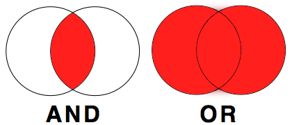
Simple Example: Just imagine, you have data of men and women who are either blond or dark-haired.
If you wanted to filter everyone who has blond hair AND is a man, all your data looks like this:
Whereas, if you wanted to filter out everyone who has either dark hair OR is a woman, you would get:
What does that mean for our student mental health data?
For example, to filter rows containing only international students who have a total acculturative stress score of more than 72, you would code:
short_MH72_inter <- filter(short_MH, inter_dom == "Inter", ToAS > 72)
glimpse(short_MH72_inter)
## Observations: 109
## Variables: 15
## $ ID <dbl> 1, 4, 5, 6, 8, 9, 11, 12, 15, 16, 23, 24, 25, 27, 28, 32,...
## $ inter_dom <chr> "Inter", "Inter", "Inter", "Inter", "Inter", "Inter", "In...
## $ Gender <chr> "Male", "Female", "Female", "Male", "Female", "Female", "...
## $ Academic <chr> "Grad", "Grad", "Grad", "Grad", "Grad", "Grad", "Grad", "...
## $ Age <dbl> 24, 29, 28, 24, 30, 25, 28, 31, 31, 30, 19, 20, 29, 30, 1...
## $ ToDep <dbl> 0, 3, 3, 6, 9, 7, 5, 8, 9, 6, 13, 1, 8, 13, 9, 9, 9, 15, ...
## $ ToSC <dbl> 34, 37, 37, 38, 41, 36, 32, 47, 31, 40, 25, 34, 39, 42, 3...
## $ APD <dbl> 23, 16, 15, 18, 16, 22, 24, 17, 23, 19, 25, 24, 18, 23, 1...
## $ AHome <dbl> 9, 10, 12, 8, 20, 12, 8, 12, 16, 9, 16, 16, 8, 15, 9, 8, ...
## $ APH <dbl> 11, 10, 5, 10, 19, 13, 10, 14, 15, 5, 10, 15, 10, 11, 10,...
## $ Afear <dbl> 8, 8, 8, 8, 15, 13, 8, 13, 8, 4, 11, 12, 8, 9, 11, 8, 8, ...
## $ ACS <dbl> 11, 6, 7, 7, 11, 10, 6, 9, 12, 13, 6, 11, 7, 5, 7, 6, 6, ...
## $ AGuilt <dbl> 2, 4, 4, 3, 6, 6, 6, 4, 8, 2, 4, 8, 4, 2, 6, 4, 4, 8, 4, ...
## $ AMiscell <dbl> 27, 21, 31, 29, 40, 33, 30, 26, 30, 22, 22, 37, 23, 26, 2...
## $ ToAS <dbl> 91, 75, 82, 83, 127, 109, 92, 95, 112, 74, 94, 123, 78, 9...
You could have also used the logical operator & (AND) instead of the comma. filter(short_MH, inter_dom == “Inter” & ToAS > 72) would have given you the same result as above.
If we wanted to filter the data short_MH for either international students OR students with total acculturative stress scores of more than 72, we could use the logical operator | (OR).
short_MH72_inter_or <- filter(short_MH, inter_dom == "Inter" | ToAS > 72)
glimpse(short_MH72_inter_or)
## Observations: 223
## Variables: 15
## $ ID <dbl> 1, 2, 3, 4, 5, 6, 7, 8, 9, 10, 11, 12, 13, 14, 15, 16, 17...
## $ inter_dom <chr> "Inter", "Inter", "Inter", "Inter", "Inter", "Inter", "In...
## $ Gender <chr> "Male", "Male", "Male", "Female", "Female", "Male", "Male...
## $ Academic <chr> "Grad", "Grad", "Grad", "Grad", "Grad", "Grad", "Grad", "...
## $ Age <dbl> 24, 28, 25, 29, 28, 24, 23, 30, 25, 31, 28, 31, 29, 23, 3...
## $ ToDep <dbl> 0, 2, 2, 3, 3, 6, 3, 9, 7, 3, 5, 8, 1, 3, 9, 6, 3, 3, 7, ...
## $ ToSC <dbl> 34, 48, 41, 37, 37, 38, 46, 41, 36, 48, 32, 47, 48, 32, 3...
## $ APD <dbl> 23, 8, 13, 16, 15, 18, 17, 16, 22, 8, 24, 17, 8, 9, 23, 1...
## $ AHome <dbl> 9, 7, 4, 10, 12, 8, 6, 20, 12, 4, 8, 12, 11, 8, 16, 9, 13...
## $ APH <dbl> 11, 5, 7, 10, 5, 10, 10, 19, 13, 5, 10, 14, 5, 5, 15, 5, ...
## $ Afear <dbl> 8, 4, 6, 8, 8, 8, 5, 15, 13, 12, 8, 13, 4, 4, 8, 4, 4, 4,...
## $ ACS <dbl> 11, 3, 4, 6, 7, 7, 3, 11, 10, 3, 6, 9, 7, 6, 12, 13, 8, 3...
## $ AGuilt <dbl> 2, 2, 3, 4, 4, 3, 2, 6, 6, 2, 6, 4, 2, 7, 8, 2, 5, 2, 2, ...
## $ AMiscell <dbl> 27, 10, 14, 21, 31, 29, 15, 40, 33, 17, 30, 26, 17, 18, 3...
## $ ToAS <dbl> 91, 39, 51, 75, 82, 83, 58, 127, 109, 51, 92, 95, 54, 57,...As you will have noticed, short_MH72_inter_or has now observations for participants that are either international students, or students with a ToAS of larger than 72. Undoubtedly, some will fall into both categories, however, participants that fit neither criterion are excluded.
Question Time
How many rows (or observations) does the object short_MH72 contain?
How many participants in this study were international students?
How many observations would the code filter(short_MH, inter_dom == "inter") return?
How many participants in this study were international students with a ToAS of more than 72?
How many participants in this study were either international students OR had a ToAS of more than 72?
If you need to filter through many different values from the same column, you can use the match operator %in%. It returns a logical value of TRUE when it detects a match and FALSE if not. Let’s make that a bit more applicable. Say we wanted to make a tibble called short_MH_age that takes the data short_MH and only keeps information from students when their Age is either 17, 20, 25, or 30.
short_MH_age <- filter(short_MH, Age %in% c(17, 20, 25, 30))You could use the OR operator here as well, but it would be pretty tedious to type out.
Your turn
Make a tibble called short_MH_ToDep that list every participant from short_MH with a ToDep score of 0, 5, 8, 15, 17, and 25.
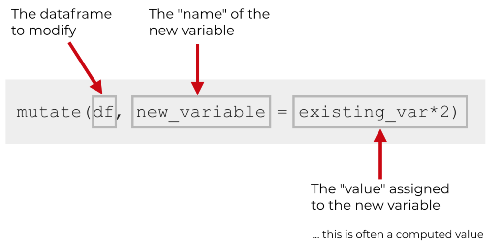
short_MH_ToDep <- filter(short_MH, ToDep %in% c(0, 5, 8, 15, 17, 25))3.6 mutate()
The mutate() function creates new variables (columns) onto the existing object. The first argument to this function is an object from your Global Environment (for example short_MH we created earlier) and the subsequent argument is the new column name and what you want it to contain. The following image was downloaded from https://www.sharpsightlabs.com/blog/mutate-in-r/
Let’s apply this to this to our short_MH data tibble. Say we wanted to create a new column Age_double that shows us the age of our participants if they are twice as old as they are now. We will save this as a new object short_MH_ext to our Global Environment rather than overwriting short_MH so that we can compare short_MH with the extended short_MH_ext later on.
short_MH_ext <- mutate(short_MH, Age_double = Age*2)
glimpse(short_MH_ext)
## Observations: 268
## Variables: 16
## $ ID <dbl> 1, 2, 3, 4, 5, 6, 7, 8, 9, 10, 11, 12, 13, 14, 15, 16, 1...
## $ inter_dom <chr> "Inter", "Inter", "Inter", "Inter", "Inter", "Inter", "I...
## $ Gender <chr> "Male", "Male", "Male", "Female", "Female", "Male", "Mal...
## $ Academic <chr> "Grad", "Grad", "Grad", "Grad", "Grad", "Grad", "Grad", ...
## $ Age <dbl> 24, 28, 25, 29, 28, 24, 23, 30, 25, 31, 28, 31, 29, 23, ...
## $ ToDep <dbl> 0, 2, 2, 3, 3, 6, 3, 9, 7, 3, 5, 8, 1, 3, 9, 6, 3, 3, 7,...
## $ ToSC <dbl> 34, 48, 41, 37, 37, 38, 46, 41, 36, 48, 32, 47, 48, 32, ...
## $ APD <dbl> 23, 8, 13, 16, 15, 18, 17, 16, 22, 8, 24, 17, 8, 9, 23, ...
## $ AHome <dbl> 9, 7, 4, 10, 12, 8, 6, 20, 12, 4, 8, 12, 11, 8, 16, 9, 1...
## $ APH <dbl> 11, 5, 7, 10, 5, 10, 10, 19, 13, 5, 10, 14, 5, 5, 15, 5,...
## $ Afear <dbl> 8, 4, 6, 8, 8, 8, 5, 15, 13, 12, 8, 13, 4, 4, 8, 4, 4, 4...
## $ ACS <dbl> 11, 3, 4, 6, 7, 7, 3, 11, 10, 3, 6, 9, 7, 6, 12, 13, 8, ...
## $ AGuilt <dbl> 2, 2, 3, 4, 4, 3, 2, 6, 6, 2, 6, 4, 2, 7, 8, 2, 5, 2, 2,...
## $ AMiscell <dbl> 27, 10, 14, 21, 31, 29, 15, 40, 33, 17, 30, 26, 17, 18, ...
## $ ToAS <dbl> 91, 39, 51, 75, 82, 83, 58, 127, 109, 51, 92, 95, 54, 57...
## $ Age_double <dbl> 48, 56, 50, 58, 56, 48, 46, 60, 50, 62, 56, 62, 58, 46, ...As we can see, short_MH_ext has one column more than short_MH. So mutate() took the value in the cells for each row of the variable Age, multiplied it by 2, and added it to the new column Age_double.
Importantly, new variables will overwrite existing variables if column headings are identical. So if we wanted to halve the values in column Age_double and store them in a column Age_double, the original Age_double would be overwritten.
short_MH_ext <- mutate(short_MH_ext, Age_double = Age_double/2)
glimpse(short_MH_ext)
## Observations: 268
## Variables: 16
## $ ID <dbl> 1, 2, 3, 4, 5, 6, 7, 8, 9, 10, 11, 12, 13, 14, 15, 16, 1...
## $ inter_dom <chr> "Inter", "Inter", "Inter", "Inter", "Inter", "Inter", "I...
## $ Gender <chr> "Male", "Male", "Male", "Female", "Female", "Male", "Mal...
## $ Academic <chr> "Grad", "Grad", "Grad", "Grad", "Grad", "Grad", "Grad", ...
## $ Age <dbl> 24, 28, 25, 29, 28, 24, 23, 30, 25, 31, 28, 31, 29, 23, ...
## $ ToDep <dbl> 0, 2, 2, 3, 3, 6, 3, 9, 7, 3, 5, 8, 1, 3, 9, 6, 3, 3, 7,...
## $ ToSC <dbl> 34, 48, 41, 37, 37, 38, 46, 41, 36, 48, 32, 47, 48, 32, ...
## $ APD <dbl> 23, 8, 13, 16, 15, 18, 17, 16, 22, 8, 24, 17, 8, 9, 23, ...
## $ AHome <dbl> 9, 7, 4, 10, 12, 8, 6, 20, 12, 4, 8, 12, 11, 8, 16, 9, 1...
## $ APH <dbl> 11, 5, 7, 10, 5, 10, 10, 19, 13, 5, 10, 14, 5, 5, 15, 5,...
## $ Afear <dbl> 8, 4, 6, 8, 8, 8, 5, 15, 13, 12, 8, 13, 4, 4, 8, 4, 4, 4...
## $ ACS <dbl> 11, 3, 4, 6, 7, 7, 3, 11, 10, 3, 6, 9, 7, 6, 12, 13, 8, ...
## $ AGuilt <dbl> 2, 2, 3, 4, 4, 3, 2, 6, 6, 2, 6, 4, 2, 7, 8, 2, 5, 2, 2,...
## $ AMiscell <dbl> 27, 10, 14, 21, 31, 29, 15, 40, 33, 17, 30, 26, 17, 18, ...
## $ ToAS <dbl> 91, 39, 51, 75, 82, 83, 58, 127, 109, 51, 92, 95, 54, 57...
## $ Age_double <dbl> 24, 28, 25, 29, 28, 24, 23, 30, 25, 31, 28, 31, 29, 23, ...So now, short_MH_ext did not gain a column (it still contains 16 variables), and Age_double has now the same values as column Age.
The main take-away message here is to always check your data after manipulation if the outcome is really what you would expected. If you don’t inspect and accidentally overwrite columns, you would not notice any difference.
No need to keep column Age_double anymore; we could just drop it. And we are back to 15 variable columns.
short_MH_ext <- mutate(short_MH_ext, Age_double = NULL)
glimpse(short_MH_ext)
## Observations: 268
## Variables: 15
## $ ID <dbl> 1, 2, 3, 4, 5, 6, 7, 8, 9, 10, 11, 12, 13, 14, 15, 16, 17...
## $ inter_dom <chr> "Inter", "Inter", "Inter", "Inter", "Inter", "Inter", "In...
## $ Gender <chr> "Male", "Male", "Male", "Female", "Female", "Male", "Male...
## $ Academic <chr> "Grad", "Grad", "Grad", "Grad", "Grad", "Grad", "Grad", "...
## $ Age <dbl> 24, 28, 25, 29, 28, 24, 23, 30, 25, 31, 28, 31, 29, 23, 3...
## $ ToDep <dbl> 0, 2, 2, 3, 3, 6, 3, 9, 7, 3, 5, 8, 1, 3, 9, 6, 3, 3, 7, ...
## $ ToSC <dbl> 34, 48, 41, 37, 37, 38, 46, 41, 36, 48, 32, 47, 48, 32, 3...
## $ APD <dbl> 23, 8, 13, 16, 15, 18, 17, 16, 22, 8, 24, 17, 8, 9, 23, 1...
## $ AHome <dbl> 9, 7, 4, 10, 12, 8, 6, 20, 12, 4, 8, 12, 11, 8, 16, 9, 13...
## $ APH <dbl> 11, 5, 7, 10, 5, 10, 10, 19, 13, 5, 10, 14, 5, 5, 15, 5, ...
## $ Afear <dbl> 8, 4, 6, 8, 8, 8, 5, 15, 13, 12, 8, 13, 4, 4, 8, 4, 4, 4,...
## $ ACS <dbl> 11, 3, 4, 6, 7, 7, 3, 11, 10, 3, 6, 9, 7, 6, 12, 13, 8, 3...
## $ AGuilt <dbl> 2, 2, 3, 4, 4, 3, 2, 6, 6, 2, 6, 4, 2, 7, 8, 2, 5, 2, 2, ...
## $ AMiscell <dbl> 27, 10, 14, 21, 31, 29, 15, 40, 33, 17, 30, 26, 17, 18, 3...
## $ ToAS <dbl> 91, 39, 51, 75, 82, 83, 58, 127, 109, 51, 92, 95, 54, 57,...If you want to add more than 2 columns, you can do that in a single mutate() statement. You can also add variables that are not numerical values, such as character or logical.
Let’s have a look at the column ToDep. According to the PHQ, the maximum score for that measure is 27, and patients having a score of 20 or above count as severely depressed. More information can be found on https://www.ncor.org.uk/wp-content/uploads/2012/12/Patient-Health-Questionnaire.pdf
Say we wanted to add two columns to short_MH_ext.
- Column 1 is called
max_PHQand contains the maximum score of 27 that can be achieved in the Patient Health Questionnaire - Column 2 is called
Dep_Severeand is of datatypelogical. It contains a comparison of the value inToDepwith the cut off score of 20. Values 20 and above should readTRUE, all other valuesFALSE.
short_MH_ext <- mutate(short_MH_ext, max_PHQ = 27,
                       Dep_Severe = ToDep >= 20)
glimpse(short_MH_ext)
## Observations: 268
## Variables: 17
## $ ID <dbl> 1, 2, 3, 4, 5, 6, 7, 8, 9, 10, 11, 12, 13, 14, 15, 16, 1...
## $ inter_dom <chr> "Inter", "Inter", "Inter", "Inter", "Inter", "Inter", "I...
## $ Gender <chr> "Male", "Male", "Male", "Female", "Female", "Male", "Mal...
## $ Academic <chr> "Grad", "Grad", "Grad", "Grad", "Grad", "Grad", "Grad", ...
## $ Age <dbl> 24, 28, 25, 29, 28, 24, 23, 30, 25, 31, 28, 31, 29, 23, ...
## $ ToDep <dbl> 0, 2, 2, 3, 3, 6, 3, 9, 7, 3, 5, 8, 1, 3, 9, 6, 3, 3, 7,...
## $ ToSC <dbl> 34, 48, 41, 37, 37, 38, 46, 41, 36, 48, 32, 47, 48, 32, ...
## $ APD <dbl> 23, 8, 13, 16, 15, 18, 17, 16, 22, 8, 24, 17, 8, 9, 23, ...
## $ AHome <dbl> 9, 7, 4, 10, 12, 8, 6, 20, 12, 4, 8, 12, 11, 8, 16, 9, 1...
## $ APH <dbl> 11, 5, 7, 10, 5, 10, 10, 19, 13, 5, 10, 14, 5, 5, 15, 5,...
## $ Afear <dbl> 8, 4, 6, 8, 8, 8, 5, 15, 13, 12, 8, 13, 4, 4, 8, 4, 4, 4...
## $ ACS <dbl> 11, 3, 4, 6, 7, 7, 3, 11, 10, 3, 6, 9, 7, 6, 12, 13, 8, ...
## $ AGuilt <dbl> 2, 2, 3, 4, 4, 3, 2, 6, 6, 2, 6, 4, 2, 7, 8, 2, 5, 2, 2,...
## $ AMiscell <dbl> 27, 10, 14, 21, 31, 29, 15, 40, 33, 17, 30, 26, 17, 18, ...
## $ ToAS <dbl> 91, 39, 51, 75, 82, 83, 58, 127, 109, 51, 92, 95, 54, 57...
## $ max_PHQ <dbl> 27, 27, 27, 27, 27, 27, 27, 27, 27, 27, 27, 27, 27, 27, ...
## $ Dep_Severe <lgl> FALSE, FALSE, FALSE, FALSE, FALSE, FALSE, FALSE, FALSE, ...
For column max_PHQ, we would not have to repeat the number 27 268 times. As it’s the same number for all cells, mentioning it once sets all the values in the column to that particular number (similar to “Scotland” last week when we were creating tibbles).
Dep_Severe = ToDep >= 20 might look a bit alien to you, but remember that a single equals sign (=) is used to assign a value to a variable whereas the relational operator (>=) is used to check whether two values are equal. These can actually co-exist in one statement. Here R reads the expression as: “compare for each row whether the cell value in ToDep is equal or larger than 20. If yes, put TRUE in the new column Dep_Severe; if not, put FALSE.
There are 8 students in this data set who would categorise as severely depressed.
Your turn
-
Add a new column to
short_MH_extthat is calledTotal_Scorethat adds together the seven subscales for each observation (row). *Hint: APD + AHome + … + AMiscell would do the trick. If we have done it correctly,Total_Scoreshould have the same values asToAS. -
Add a second new column that is called
correctthat evaluates whetherTotal_ScoreandToASare identical columns.
short_MH_ext <- mutate(short_MH_ext, Total_Score = APD + AHome + APH + Afear + ACS + AGuilt + AMiscell,
                       Correct = Total_Score == ToAS)
glimpse(short_MH_ext)
## Observations: 268
## Variables: 19
## $ ID <dbl> 1, 2, 3, 4, 5, 6, 7, 8, 9, 10, 11, 12, 13, 14, 15, 16, ...
## $ inter_dom <chr> "Inter", "Inter", "Inter", "Inter", "Inter", "Inter", "...
## $ Gender <chr> "Male", "Male", "Male", "Female", "Female", "Male", "Ma...
## $ Academic <chr> "Grad", "Grad", "Grad", "Grad", "Grad", "Grad", "Grad",...
## $ Age <dbl> 24, 28, 25, 29, 28, 24, 23, 30, 25, 31, 28, 31, 29, 23,...
## $ ToDep <dbl> 0, 2, 2, 3, 3, 6, 3, 9, 7, 3, 5, 8, 1, 3, 9, 6, 3, 3, 7...
## $ ToSC <dbl> 34, 48, 41, 37, 37, 38, 46, 41, 36, 48, 32, 47, 48, 32,...
## $ APD <dbl> 23, 8, 13, 16, 15, 18, 17, 16, 22, 8, 24, 17, 8, 9, 23,...
## $ AHome <dbl> 9, 7, 4, 10, 12, 8, 6, 20, 12, 4, 8, 12, 11, 8, 16, 9, ...
## $ APH <dbl> 11, 5, 7, 10, 5, 10, 10, 19, 13, 5, 10, 14, 5, 5, 15, 5...
## $ Afear <dbl> 8, 4, 6, 8, 8, 8, 5, 15, 13, 12, 8, 13, 4, 4, 8, 4, 4, ...
## $ ACS <dbl> 11, 3, 4, 6, 7, 7, 3, 11, 10, 3, 6, 9, 7, 6, 12, 13, 8,...
## $ AGuilt <dbl> 2, 2, 3, 4, 4, 3, 2, 6, 6, 2, 6, 4, 2, 7, 8, 2, 5, 2, 2...
## $ AMiscell <dbl> 27, 10, 14, 21, 31, 29, 15, 40, 33, 17, 30, 26, 17, 18,...
## $ ToAS <dbl> 91, 39, 51, 75, 82, 83, 58, 127, 109, 51, 92, 95, 54, 5...
## $ max_PHQ <dbl> 27, 27, 27, 27, 27, 27, 27, 27, 27, 27, 27, 27, 27, 27,...
## $ Dep_Severe <lgl> FALSE, FALSE, FALSE, FALSE, FALSE, FALSE, FALSE, FALSE,...
## $ Total_Score <dbl> 91, 39, 51, 75, 82, 83, 58, 127, 109, 51, 92, 95, 54, 5...
## $ Correct <lgl> TRUE, TRUE, TRUE, TRUE, TRUE, TRUE, TRUE, TRUE, TRUE, T...Follow-up Question
Although the last examples are useful to illustrate how mutate() works, you do not need two identical columns. Using one of today’s dplyr functions, remove the columns Total_Score and Correct from the dataset short_MH_ext. Save this as a new object short_MH_ext2 to your Global Environment.
short_MH_ext2 <- mutate(short_MH_ext, Total_Score = NULL,
                       Correct = NULL)
glimpse(short_MH_ext2)
## Observations: 268
## Variables: 17
## $ ID <dbl> 1, 2, 3, 4, 5, 6, 7, 8, 9, 10, 11, 12, 13, 14, 15, 16, 1...
## $ inter_dom <chr> "Inter", "Inter", "Inter", "Inter", "Inter", "Inter", "I...
## $ Gender <chr> "Male", "Male", "Male", "Female", "Female", "Male", "Mal...
## $ Academic <chr> "Grad", "Grad", "Grad", "Grad", "Grad", "Grad", "Grad", ...
## $ Age <dbl> 24, 28, 25, 29, 28, 24, 23, 30, 25, 31, 28, 31, 29, 23, ...
## $ ToDep <dbl> 0, 2, 2, 3, 3, 6, 3, 9, 7, 3, 5, 8, 1, 3, 9, 6, 3, 3, 7,...
## $ ToSC <dbl> 34, 48, 41, 37, 37, 38, 46, 41, 36, 48, 32, 47, 48, 32, ...
## $ APD <dbl> 23, 8, 13, 16, 15, 18, 17, 16, 22, 8, 24, 17, 8, 9, 23, ...
## $ AHome <dbl> 9, 7, 4, 10, 12, 8, 6, 20, 12, 4, 8, 12, 11, 8, 16, 9, 1...
## $ APH <dbl> 11, 5, 7, 10, 5, 10, 10, 19, 13, 5, 10, 14, 5, 5, 15, 5,...
## $ Afear <dbl> 8, 4, 6, 8, 8, 8, 5, 15, 13, 12, 8, 13, 4, 4, 8, 4, 4, 4...
## $ ACS <dbl> 11, 3, 4, 6, 7, 7, 3, 11, 10, 3, 6, 9, 7, 6, 12, 13, 8, ...
## $ AGuilt <dbl> 2, 2, 3, 4, 4, 3, 2, 6, 6, 2, 6, 4, 2, 7, 8, 2, 5, 2, 2,...
## $ AMiscell <dbl> 27, 10, 14, 21, 31, 29, 15, 40, 33, 17, 30, 26, 17, 18, ...
## $ ToAS <dbl> 91, 39, 51, 75, 82, 83, 58, 127, 109, 51, 92, 95, 54, 57...
## $ max_PHQ <dbl> 27, 27, 27, 27, 27, 27, 27, 27, 27, 27, 27, 27, 27, 27, ...
## $ Dep_Severe <lgl> FALSE, FALSE, FALSE, FALSE, FALSE, FALSE, FALSE, FALSE, ...
You could have also used the function select() to drop or select variable columns. For example:
-
select(short_MH_ext, ID:Dep_Severe) or
- select(short_MH_ext, -Total_Score, -Correct)
3.7 Formative Homework
The folder for the formative assessment can now be downloaded from moodle.
- Load
tidyverseinto the library. - Read the data from
TraitJudgementData.csvinto yourGlobal Environmentas an object calledtraits_data. - Look at the data. Familiarise yourself with the data (see next section, and the paper in the folder), as well as the datatypes of each column.
3.7.1 Brief introduction to the homework data
For the homework assignments each week, we will be using an open access dataset into how personality is determined from voices. A full version of the paper can be found https://journals.plos.org/plosone/article?id=10.1371/journal.pone.0204991. All data and sounds are available on OSF (osf.io/s3cxy).
However, for your assignment this week, all files necessary are compiled in a folder to download from moodle.
The data in the TraitJudgementData.csv has ratings on 3 different personality traits (Trustworthiness, Dominance, and Attractiveness) for 30 male and 30 female voice stimuli. In total, 181 participants rated either male OR female speakers on ONE personality trait (e.g. Trustworthiness) only. The speakers were judged after saying a socially relevant word (“Hello”), a socially ambiguous word (“Colors”), a socially relevant sentence (“I urge you to submit your essay by the end of the week”), and a socially ambiguous sentence (“Some have accepted it as a miracle without physical explanation”). Socially relevant stimuli were meant to address the listener, whereas socially ambiguous stimuli were intended to not be directed towards the listener. Each participant rated all the voice stimuli twice in all four conditions (socially relevant words (RW), socially relevant sentences (RS), socially ambiguous words (AW), and socially ambiguous sentences (AS)). The experiment was conducted online.
Here is a brief summary overview of the columns in the TraitJudgementData.csv.
| column name | description |
|---|---|
| PP_ID | Participant’s ID |
| PP_Age | Participant’s Age |
| PP_Sex | Participant’s Sex (“female”, “male”) |
| Nationality | Participant’s Nationality |
| Trait | Personality Trait participant judged the vocal stimuli on (“Trustworthiness”, “Dominance”, “Attractiveness”) |
| Voice | Speaker’s ID |
| Voice_Sex | Speaker’s Sex (“Female”, “Male”) |
| Condition | Speaker’s recording of socially relevant words (“RW”), socially relevant sentences (“RS”), socially ambiguous words (“AW”), and socially ambiguous sentences (“AS”) |
| Rating | Participants rated each Voice in each Condition twice (“Rating1”, “Rating2”) |
| Response | Participant’s Trait judgements on a scale from 1 - 500 |
| Reaction | Participant’s Reaction Time |