Chapter 4 Data Transformation 2: More One and Two Table Verbs
Intended Learning Outcomes
- Be able to use the following dplyr one-table verbs:
- group_by()
- summarise()
Be able to chain functions together using the pipe operator (%>%)
Be able to use the following dplyr two-table verbs:
- Mutating joins:
left_join(),right_join(),full_join(),inner_join() - Binding joins:
bind_rows(),bind_cols()
This lesson is led by Kate Haining.
4.1 Pre-Steps
- Set your working directory to the
L3L4_datafolder we were working with last week and that contains the data filesStudent_Mental_Health.csvandAnx_Emp.csv. - Open the
L3L4_stubfile. - Load
tidyverseinto the library. - Read the data from
Student_Mental_Health.csvinto yourGlobal Environmentasstudent_MH. - Deselect the columns
Region,Stay_Cate,Japanese_cate, andEnglish_cate. Store this data as an objectshort_MH. - Read the data from
Anx_Emp.csvinto yourGlobal Environmentasextra_MH. This data will be needed for the two-table verbs later on.Anx_Emp.csvcontains fake data relating to 267 students in the previous data file (short_MH). The columnGAD7refers to students’ scores on the Generalized Anxiety Disorder 7-item (GAD-7) questionnaire and the columnEmploymentoutlines the students’ employment status i.e. part-time, full-time or unemployed.
library(tidyverse)
student_MH <- read_csv("Student_Mental_Health.csv")
short_MH <- select(student_MH, -Region, -Stay_Cate, -Japanese_cate, -English_cate)
extra_MH <- read_csv("Anx_Emp.csv")
4.2 group_by() and summarise()
In order to compute summary statistics such as mean, median and standard deviation, use the summarise() function. The first argument to this function is the object short_MH and the subsequent argument is the new column name and what mathematical operation you want it to contain. You can add as many summary statistics in one summarise() function as you want; just separate them by a comma. For example, say you wanted to work out the mean total score of depression and accompanying standard deviation for the entire sample:
short_MH_ToDep <- summarise(short_MH, mean = mean(ToDep), sd = sd(ToDep))
short_MH_ToDep
## # A tibble: 1 x 2
## mean sd
## <dbl> <dbl>
## 1 8.19 4.95Therefore, the mean total score of depression is 8.19 with a standard deviation of 4.95. It would be interesting to break these summary statistics down into subsets for example ToDep for the males and females separately. This is where the group_by() function comes in handy. It can organise observations (rows) by variables (columns) such as Gender. The first argument to this function is the object you created last week (short_MH) and the subsequent argument is the variable you want to group by:
short_MH_gen <- group_by(short_MH, Gender)If you view the object short_MH_gen, it will not look any different to the original dataset (short_MH). However, be aware that the underlying structure has changed. In fact, you could type glimpse(short_MH_gen) to double check this.
glimpse(short_MH_gen)## Observations: 268
## Variables: 15
## Groups: Gender [2]
## $ ID <dbl> 1, 2, 3, 4, 5, 6, 7, 8, 9, 10, 11, 12, 13, 14, 15, 16, 17...
## $ inter_dom <chr> "Inter", "Inter", "Inter", "Inter", "Inter", "Inter", "In...
## $ Gender <chr> "Male", "Male", "Male", "Female", "Female", "Male", "Male...
## $ Academic <chr> "Grad", "Grad", "Grad", "Grad", "Grad", "Grad", "Grad", "...
## $ Age <dbl> 24, 28, 25, 29, 28, 24, 23, 30, 25, 31, 28, 31, 29, 23, 3...
## $ ToDep <dbl> 0, 2, 2, 3, 3, 6, 3, 9, 7, 3, 5, 8, 1, 3, 9, 6, 3, 3, 7, ...
## $ ToSC <dbl> 34, 48, 41, 37, 37, 38, 46, 41, 36, 48, 32, 47, 48, 32, 3...
## $ APD <dbl> 23, 8, 13, 16, 15, 18, 17, 16, 22, 8, 24, 17, 8, 9, 23, 1...
## $ AHome <dbl> 9, 7, 4, 10, 12, 8, 6, 20, 12, 4, 8, 12, 11, 8, 16, 9, 13...
## $ APH <dbl> 11, 5, 7, 10, 5, 10, 10, 19, 13, 5, 10, 14, 5, 5, 15, 5, ...
## $ Afear <dbl> 8, 4, 6, 8, 8, 8, 5, 15, 13, 12, 8, 13, 4, 4, 8, 4, 4, 4,...
## $ ACS <dbl> 11, 3, 4, 6, 7, 7, 3, 11, 10, 3, 6, 9, 7, 6, 12, 13, 8, 3...
## $ AGuilt <dbl> 2, 2, 3, 4, 4, 3, 2, 6, 6, 2, 6, 4, 2, 7, 8, 2, 5, 2, 2, ...
## $ AMiscell <dbl> 27, 10, 14, 21, 31, 29, 15, 40, 33, 17, 30, 26, 17, 18, 3...
## $ ToAS <dbl> 91, 39, 51, 75, 82, 83, 58, 127, 109, 51, 92, 95, 54, 57,...You can now feed this grouped dataset (short_MH_gen) into the previous code line to obtain summary statistics by Gender:
short_MH_ToDep_gen <- summarise(short_MH_gen, mean = mean(ToDep), sd = sd(ToDep))
short_MH_ToDep_gen
## # A tibble: 2 x 3
## Gender mean sd
## <chr> <dbl> <dbl>
## 1 Female 8.4 4.67
## 2 Male 7.82 5.42Question Time
What gender has the highest mean total score of depression?
You might also want to calculate and display the number of males and females in the dataset. This can be achieved by adding the summary function n() to your previous code line:
short_MH_ToDep_gen <- summarise(short_MH_gen, n = n(), mean = mean(ToDep), sd = sd(ToDep))
short_MH_ToDep_gen
## # A tibble: 2 x 4
## Gender n mean sd
## <chr> <int> <dbl> <dbl>
## 1 Female 170 8.4 4.67
## 2 Male 98 7.82 5.42Question Time
How many males are in the dataset?
How many females are in the dataset?
Finally, it is possible to add multiple grouping variables. For example, the following code groups short_MH by Gender and Academic level and then calculates the mean total score of depression (ToDep) for male and female graduates and undergraduates (4 groups).
short_MH_group <- group_by(short_MH, Gender, Academic)
short_MH_ToDep_group <- summarise(short_MH_group, mean = mean(ToDep))
short_MH_ToDep_group
## # A tibble: 4 x 3
## # Groups: Gender [2]
## Gender Academic mean
## <chr> <chr> <dbl>
## 1 Female Grad 7
## 2 Female Under 8.52
## 3 Male Grad 2.5
## 4 Male Under 8.29Question Time
Which group appears to be most resilient to depression?
Luckily for you, the dataset does not contain any missing values, denoted NA in R. Missing values are always a bit of a hassle to deal with. Any computation you do that involves NA returns an NA - which translates as “you will not get a numeric result when your column contains missing values”. Missing values can be removed by adding the argument na.rm = TRUE to calculation functions like mean(), median() or sd(). For example, the previous code line would read:
short_MH_ToDep_group <- summarise(short_MH_group, mean = mean(ToDep, na.rm = TRUE))
If you need to return the data to a non-grouped form, use the ungroup() function.
glimpse(short_MH_gen)## Observations: 268
## Variables: 15
## Groups: Gender [2]
## $ ID <dbl> 1, 2, 3, 4, 5, 6, 7, 8, 9, 10, 11, 12, 13, 14, 15, 16, 17...
## $ inter_dom <chr> "Inter", "Inter", "Inter", "Inter", "Inter", "Inter", "In...
## $ Gender <chr> "Male", "Male", "Male", "Female", "Female", "Male", "Male...
## $ Academic <chr> "Grad", "Grad", "Grad", "Grad", "Grad", "Grad", "Grad", "...
## $ Age <dbl> 24, 28, 25, 29, 28, 24, 23, 30, 25, 31, 28, 31, 29, 23, 3...
## $ ToDep <dbl> 0, 2, 2, 3, 3, 6, 3, 9, 7, 3, 5, 8, 1, 3, 9, 6, 3, 3, 7, ...
## $ ToSC <dbl> 34, 48, 41, 37, 37, 38, 46, 41, 36, 48, 32, 47, 48, 32, 3...
## $ APD <dbl> 23, 8, 13, 16, 15, 18, 17, 16, 22, 8, 24, 17, 8, 9, 23, 1...
## $ AHome <dbl> 9, 7, 4, 10, 12, 8, 6, 20, 12, 4, 8, 12, 11, 8, 16, 9, 13...
## $ APH <dbl> 11, 5, 7, 10, 5, 10, 10, 19, 13, 5, 10, 14, 5, 5, 15, 5, ...
## $ Afear <dbl> 8, 4, 6, 8, 8, 8, 5, 15, 13, 12, 8, 13, 4, 4, 8, 4, 4, 4,...
## $ ACS <dbl> 11, 3, 4, 6, 7, 7, 3, 11, 10, 3, 6, 9, 7, 6, 12, 13, 8, 3...
## $ AGuilt <dbl> 2, 2, 3, 4, 4, 3, 2, 6, 6, 2, 6, 4, 2, 7, 8, 2, 5, 2, 2, ...
## $ AMiscell <dbl> 27, 10, 14, 21, 31, 29, 15, 40, 33, 17, 30, 26, 17, 18, 3...
## $ ToAS <dbl> 91, 39, 51, 75, 82, 83, 58, 127, 109, 51, 92, 95, 54, 57,...short_MH_gen <- ungroup(short_MH_gen)
glimpse(short_MH_gen)## Observations: 268
## Variables: 15
## $ ID <dbl> 1, 2, 3, 4, 5, 6, 7, 8, 9, 10, 11, 12, 13, 14, 15, 16, 17...
## $ inter_dom <chr> "Inter", "Inter", "Inter", "Inter", "Inter", "Inter", "In...
## $ Gender <chr> "Male", "Male", "Male", "Female", "Female", "Male", "Male...
## $ Academic <chr> "Grad", "Grad", "Grad", "Grad", "Grad", "Grad", "Grad", "...
## $ Age <dbl> 24, 28, 25, 29, 28, 24, 23, 30, 25, 31, 28, 31, 29, 23, 3...
## $ ToDep <dbl> 0, 2, 2, 3, 3, 6, 3, 9, 7, 3, 5, 8, 1, 3, 9, 6, 3, 3, 7, ...
## $ ToSC <dbl> 34, 48, 41, 37, 37, 38, 46, 41, 36, 48, 32, 47, 48, 32, 3...
## $ APD <dbl> 23, 8, 13, 16, 15, 18, 17, 16, 22, 8, 24, 17, 8, 9, 23, 1...
## $ AHome <dbl> 9, 7, 4, 10, 12, 8, 6, 20, 12, 4, 8, 12, 11, 8, 16, 9, 13...
## $ APH <dbl> 11, 5, 7, 10, 5, 10, 10, 19, 13, 5, 10, 14, 5, 5, 15, 5, ...
## $ Afear <dbl> 8, 4, 6, 8, 8, 8, 5, 15, 13, 12, 8, 13, 4, 4, 8, 4, 4, 4,...
## $ ACS <dbl> 11, 3, 4, 6, 7, 7, 3, 11, 10, 3, 6, 9, 7, 6, 12, 13, 8, 3...
## $ AGuilt <dbl> 2, 2, 3, 4, 4, 3, 2, 6, 6, 2, 6, 4, 2, 7, 8, 2, 5, 2, 2, ...
## $ AMiscell <dbl> 27, 10, 14, 21, 31, 29, 15, 40, 33, 17, 30, 26, 17, 18, 3...
## $ ToAS <dbl> 91, 39, 51, 75, 82, 83, 58, 127, 109, 51, 92, 95, 54, 57,...4.3 The pipe operator (%>%)
As you may have noticed, your environment pane has become increasingly cluttered. Indeed, every time you introduced a new line of code, you created a uniquely-named object (unless your original object is overwritten). This can become confusing and time-consuming. One solution is the pipe operator (%>%) which aims to increase efficiency and improve the readability of your code. The pipe operator (%>%) read as “and then” allows you to chain functions together, eliminating the need to create intermediary objects. There is no limit as to how many functions you can chain together in a single pipeline.
For example, in order to select(), arrange(), group_by() and summarise() the data, you used the following code lines:
short_MH <- select(student_MH, -Region, -Stay_Cate, -Japanese_cate, -English_cate)
short_MH_arr <- arrange(short_MH, desc(Gender), desc(ToAS))
short_MH_group <- group_by(short_MH_arr, Gender, Academic)
short_MH_ToDep_group <- summarise(short_MH_group, mean = mean(ToDep))
short_MH_ToDep_group
## # A tibble: 4 x 3
## # Groups: Gender [2]
## Gender Academic mean
## <chr> <chr> <dbl>
## 1 Female Grad 7
## 2 Female Under 8.52
## 3 Male Grad 2.5
## 4 Male Under 8.29However, utilisation of the pipe operator (%>%) can simplify this process and create only one object (short_MH_ToDep_group2) as shown:
short_MH_ToDep_group2 <- student_MH %>%
  select(-Region, -Stay_Cate, -Japanese_cate, -English_cate) %>%
  arrange(desc(Gender), desc(ToAS)) %>%
  group_by(Gender, Academic) %>%
  summarise(mean = mean(ToDep))
short_MH_ToDep_group2
## # A tibble: 4 x 3
## # Groups: Gender [2]
## Gender Academic mean
## <chr> <chr> <dbl>
## 1 Female Grad 7
## 2 Female Under 8.52
## 3 Male Grad 2.5
## 4 Male Under 8.29As you can see, short_MH_ToDep_group2 produces the same output as short_MH_ToDep_group. So, pipes automatically take the output from one function and feed it directly to the next function. Without pipes, you needed to insert your chosen dataset as the first argument to every function. With pipes, you are only required to specify the original dataset (i.e student_MH) once at the beginning of the pipeline. You don’t need the first argument of each of the functions anymore, because the pipe will know to look at the dataset from the previous step of the pipeline.
Your turn
Amend the previous pipeline short_MH_ToDep_group2 so that
-
GenderandToASare arranged in ascending order. -
Only those observations with total social connectedness scores (
ToSC) of more than 24 are kept -
The standard deviation of values in the
ToDepcolumn is calculated for males and females at each academic level
Save this as an object called short_MH_ToDep_group3 to your Global Environment.
short_MH_ToDep_group3 <- student_MH %>%
  select(-Region, -Stay_Cate, -Japanese_cate, -English_cate) %>%
  arrange(Gender, ToAS) %>%
  filter(ToSC >25) %>%
  group_by(Gender, Academic) %>%
  summarise(mean = mean(ToDep), sd = sd(ToDep))
short_MH_ToDep_group3
## # A tibble: 4 x 4
## # Groups: Gender [2]
## Gender Academic mean sd
## <chr> <chr> <dbl> <dbl>
## 1 Female Grad 7 3.51
## 2 Female Under 7.53 3.99
## 3 Male Grad 2.5 1.77
## 4 Male Under 7.26 4.65
Note that in the above code chunk, the data object has been on its own line in the code followed immediately by %>% before starting with the “functions”.
short_MH_ToDep_group2 <- student_MH %>%
select(-Region, -Stay_Cate, -Japanese_cate, -English_cate) %>%
…
The other option would have been to put the data object as the first argument within the first function, such as
short_MH_ToDep_group2 <- select(student_MH, -Region, -Stay_Cate, -Japanese_cate, -English_cate) %>% …
The benefit of having the data on its own is that you reorder functions easily or squeeze another one in (for example if you summarised something but forgot to group beforehand) without having to remember to “move” the data object into the first argument of the chain.
4.4 Two-Table Verbs
More often than not, data scientists collect and store their data across multiple tables. In order to effectively combine multiple tables, dplyr provides a selection of two-table verbs. Today we will focus on two categories of two-table verbs - mutating join verbs and binding join verbs.
4.4.1 Mutating Join Verbs
Mutating join verbs combine the variables (columns) of two tables so that matching rows are together. There are 4 different types of mutating joins, namely inner_join(), left_join(), right_join(), and full_join().
Mutating joins have the following basic syntax:
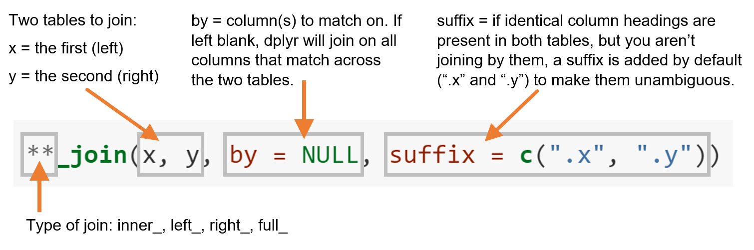
Let’s investigate joins using a simple example by creating two tibbles, data1 (shown below in blue) and data2 (shown below in green), both with only two columns, and two rows.
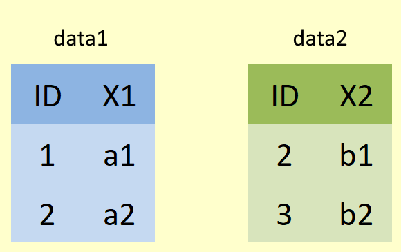
Coded in R that would look like:
data1 <- tibble(ID = 1:2,
                X1 = c("a1", "a2"))
data2 <- tibble(ID = 2:3,
                X2 = c("b1", "b2"))
For the following examples, imagine that X1 refers to student names and X2 relates to student grades. Let’s also imagine that X2 includes grades for students who have since dropped the course (and thus been removed from X1) and that X2 is missing some students who didn’t sit the exam.
4.4.1.1 inner_join()
An inner join returns all rows from x that have a match in y, whereby x is the first (left) table and y is the second (right) table. All columns from x and y are present in the merged object. If there are multiple rows that match, all of them are returned.
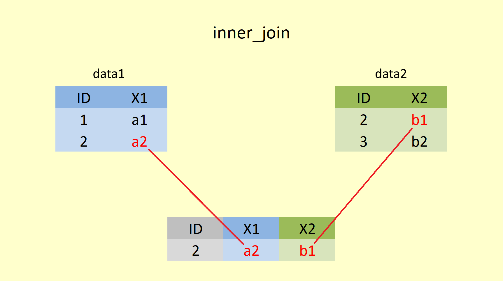
Merging data1 and data2 by inner_join() would be coded in R:
inner_join(data1, data2, by="ID")## # A tibble: 1 x 3
## ID X1 X2
## <int> <chr> <chr>
## 1 2 a2 b1Using an inner join would return only 1 row of observations because the only ID value matching in data1 and data2 is the row with ID = 2. However, we are still merging both tibbles together, meaning that all columns from data1 and data2 are kept (in our case X1 and X2). In the applied example, two students (ID 3 & 4) would be dropped from the output as their ID is only present in one table and thus, is unsuitable for matching. The inner join is useful in this situation as it ensures that grades are only held for students who still take the course and actually sat the exam.
inner_join(data1, data2) would have produced the same outcome. When the by statement is omitted, data1 and data2 are joined by ALL “overlapping” variable columns (in this case ID). Don’t believe it? Try it out in your Console!
Question Time
Let’s apply an inner join to join short_MH with extra_MH (the fake data we read in during today’s pre-steps). Before we do that, it might be wise to remind ourselves of the number of rows and columns we are dealing with in both datasets.
How many rows (or observations) does short_MH have?
How many columns (or variables) does short_MH have?
How many rows (or observations) does extra_MH have?
How many columns (or variables) does extra_MH have?
Notice that:
- Both datasets contain a common column
ID - One person (
ID = 3) is missing from the second dataset (extra_MH)
Your turn
Now join short_MH and extra_MH using inner_join(). Save your results in the Global Environment as an object called MH_inner. How many rows and columns do you think MH_inner should have?
MH_inner <- inner_join(short_MH, extra_MH, by = "ID")
glimpse(MH_inner)
## Observations: 267
## Variables: 17
## $ ID <dbl> 1, 2, 4, 5, 6, 7, 8, 9, 10, 11, 12, 13, 14, 15, 16, 17, ...
## $ inter_dom <chr> "Inter", "Inter", "Inter", "Inter", "Inter", "Inter", "I...
## $ Gender <chr> "Male", "Male", "Female", "Female", "Male", "Male", "Fem...
## $ Academic <chr> "Grad", "Grad", "Grad", "Grad", "Grad", "Grad", "Grad", ...
## $ Age <dbl> 24, 28, 29, 28, 24, 23, 30, 25, 31, 28, 31, 29, 23, 31, ...
## $ ToDep <dbl> 0, 2, 3, 3, 6, 3, 9, 7, 3, 5, 8, 1, 3, 9, 6, 3, 3, 7, 1,...
## $ ToSC <dbl> 34, 48, 37, 37, 38, 46, 41, 36, 48, 32, 47, 48, 32, 31, ...
## $ APD <dbl> 23, 8, 16, 15, 18, 17, 16, 22, 8, 24, 17, 8, 9, 23, 19, ...
## $ AHome <dbl> 9, 7, 10, 12, 8, 6, 20, 12, 4, 8, 12, 11, 8, 16, 9, 13, ...
## $ APH <dbl> 11, 5, 10, 5, 10, 10, 19, 13, 5, 10, 14, 5, 5, 15, 5, 7,...
## $ Afear <dbl> 8, 4, 8, 8, 8, 5, 15, 13, 12, 8, 13, 4, 4, 8, 4, 4, 4, 7...
## $ ACS <dbl> 11, 3, 6, 7, 7, 3, 11, 10, 3, 6, 9, 7, 6, 12, 13, 8, 3, ...
## $ AGuilt <dbl> 2, 2, 4, 4, 3, 2, 6, 6, 2, 6, 4, 2, 7, 8, 2, 5, 2, 2, 3,...
## $ AMiscell <dbl> 27, 10, 21, 31, 29, 15, 40, 33, 17, 30, 26, 17, 18, 30, ...
## $ ToAS <dbl> 91, 39, 75, 82, 83, 58, 127, 109, 51, 92, 95, 54, 57, 11...
## $ GAD7 <dbl> 8, 1, 0, 1, 14, 2, 1, 0, 2, 0, 2, 8, 0, 6, 12, 4, 0, 5, ...
## $ Employment <chr> "Unemployed", "Part", "Part", "Full", "Unemployed", "Par...
MH_inner has 267 rows, and 17 columns.
-
rows: The overlapping
IDnumbers in both dataframes are1,2,4,5…,268which makes for 267 values.
-
columns: total number of columns is 15 (from
short_MH) + 3 (fromextra_MH) - the columnIDthat exists in both objects.
Notice how no rows have missing values.
4.4.1.2 left_join()
A left join returns all rows from x, and all columns from x and y. Rows in the left table with no match in the right table will have missing values (NA) in the new columns.
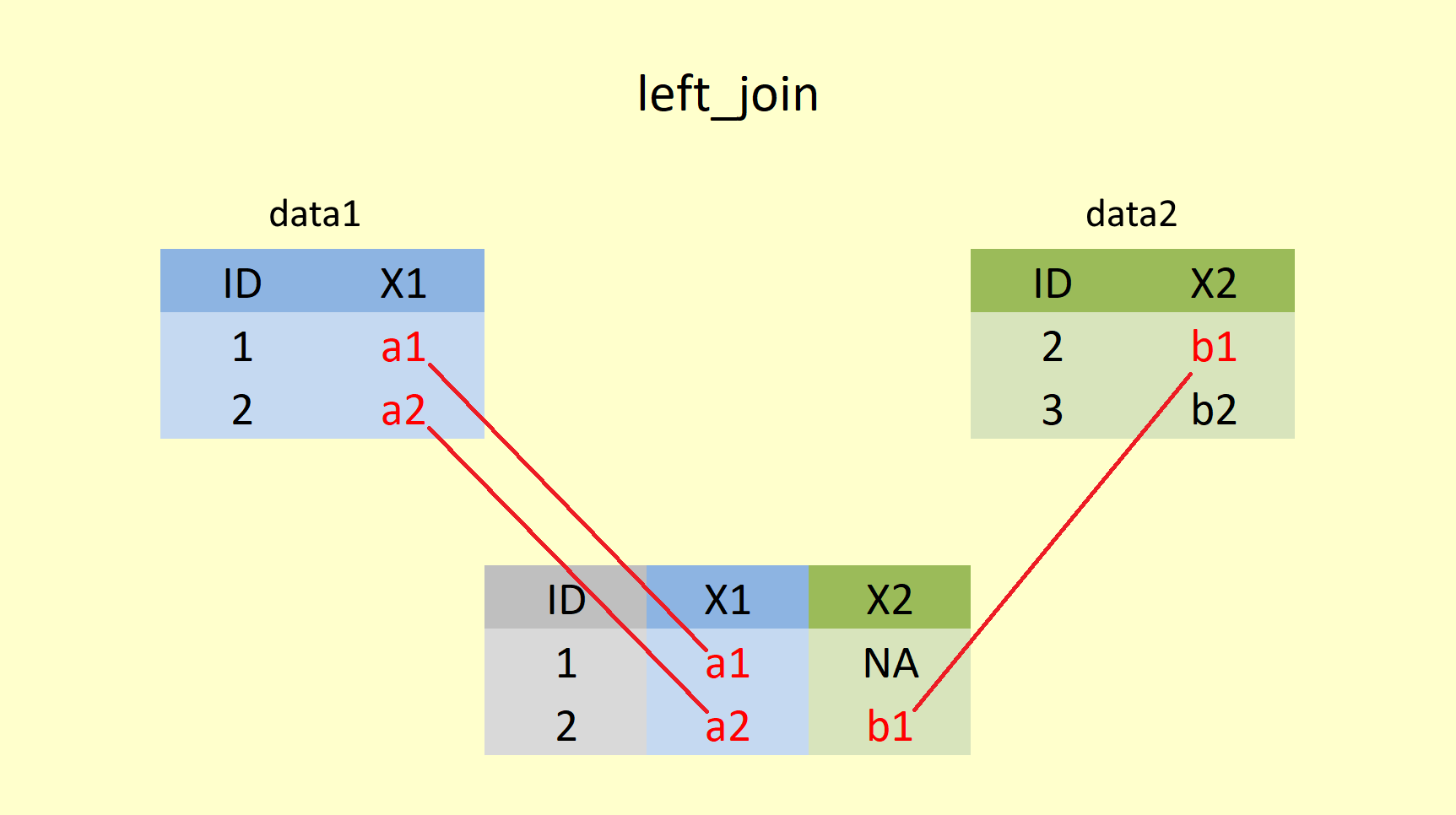
Let’s try this left_join() function for our simple example of data1 and data2 in R.
left_join(data1, data2, by="ID")## # A tibble: 2 x 3
## ID X1 X2
## <int> <chr> <chr>
## 1 1 a1 <NA>
## 2 2 a2 b1Here data1 is returned in full, and for every matching ID number, the value from data2 is added for X2. However, data2 does not have any value for ID = 1, hence NA is added in X2. The left join is useful if you want to simply append student names to student grades, regardless of whether students sat the exam or not. Students with NA values in the grade column could be offered more support and guidance in the future.
Question Time
Your turn
Combine short_MH and extra_MH using left_join(). Save your results in the Global Environment as an object called MH_left. How many rows and columns are you expecting for MH_left?
MH_left <- left_join(short_MH, extra_MH, by = "ID")
glimpse(MH_left)
## Observations: 268
## Variables: 17
## $ ID <dbl> 1, 2, 3, 4, 5, 6, 7, 8, 9, 10, 11, 12, 13, 14, 15, 16, 1...
## $ inter_dom <chr> "Inter", "Inter", "Inter", "Inter", "Inter", "Inter", "I...
## $ Gender <chr> "Male", "Male", "Male", "Female", "Female", "Male", "Mal...
## $ Academic <chr> "Grad", "Grad", "Grad", "Grad", "Grad", "Grad", "Grad", ...
## $ Age <dbl> 24, 28, 25, 29, 28, 24, 23, 30, 25, 31, 28, 31, 29, 23, ...
## $ ToDep <dbl> 0, 2, 2, 3, 3, 6, 3, 9, 7, 3, 5, 8, 1, 3, 9, 6, 3, 3, 7,...
## $ ToSC <dbl> 34, 48, 41, 37, 37, 38, 46, 41, 36, 48, 32, 47, 48, 32, ...
## $ APD <dbl> 23, 8, 13, 16, 15, 18, 17, 16, 22, 8, 24, 17, 8, 9, 23, ...
## $ AHome <dbl> 9, 7, 4, 10, 12, 8, 6, 20, 12, 4, 8, 12, 11, 8, 16, 9, 1...
## $ APH <dbl> 11, 5, 7, 10, 5, 10, 10, 19, 13, 5, 10, 14, 5, 5, 15, 5,...
## $ Afear <dbl> 8, 4, 6, 8, 8, 8, 5, 15, 13, 12, 8, 13, 4, 4, 8, 4, 4, 4...
## $ ACS <dbl> 11, 3, 4, 6, 7, 7, 3, 11, 10, 3, 6, 9, 7, 6, 12, 13, 8, ...
## $ AGuilt <dbl> 2, 2, 3, 4, 4, 3, 2, 6, 6, 2, 6, 4, 2, 7, 8, 2, 5, 2, 2,...
## $ AMiscell <dbl> 27, 10, 14, 21, 31, 29, 15, 40, 33, 17, 30, 26, 17, 18, ...
## $ ToAS <dbl> 91, 39, 51, 75, 82, 83, 58, 127, 109, 51, 92, 95, 54, 57...
## $ GAD7 <dbl> 8, 1, NA, 0, 1, 14, 2, 1, 0, 2, 0, 2, 8, 0, 6, 12, 4, 0,...
## $ Employment <chr> "Unemployed", "Part", NA, "Part", "Full", "Unemployed", ...
Remember that ID number 3 is missing from the second (right) dataset. Since the first (left) dataset is prioritised in a left_join() and data1 contains ID number 3, it is retained in the new dataset MH_left and NA is added to GAD7 and Employment.
4.4.1.3 right_join()
A right join returns all rows from y, and all columns from x and y, whereby y is the second (right table) and x is the first (left) table. Rows in the second table with no match in the first table will have NA values in the new columns.
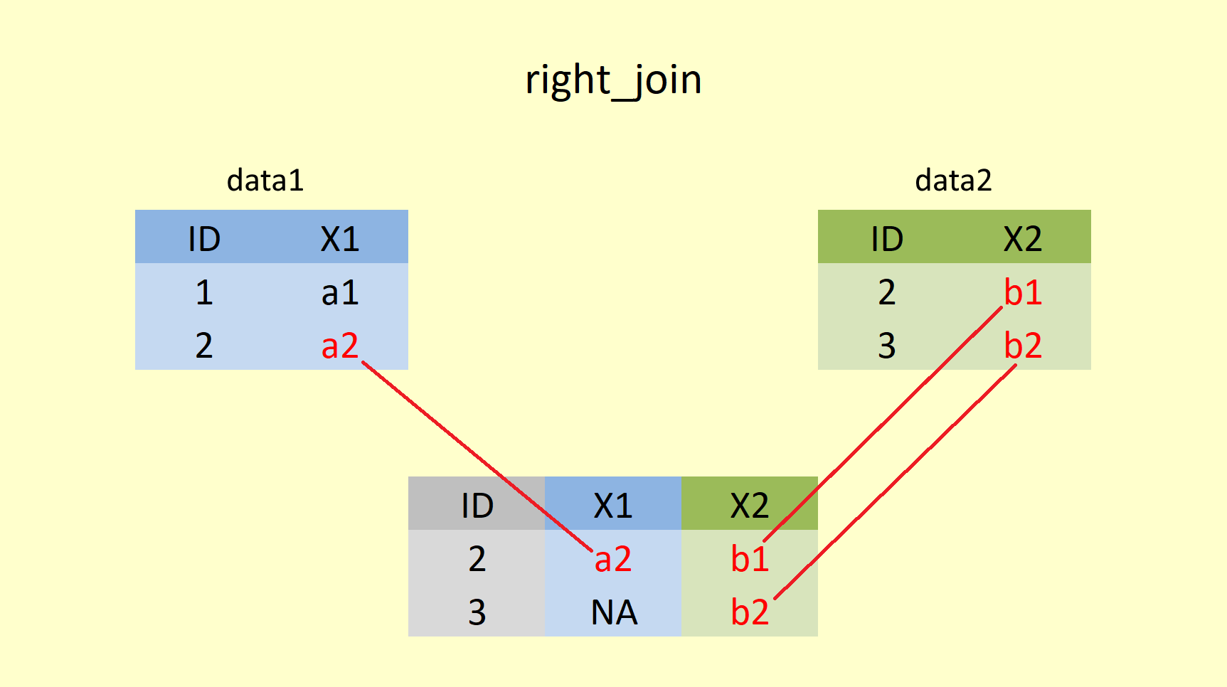
However, code-wise, you would still enter x as the first, and y as the second argument within right_join().
right_join(data1, data2, by = "ID")## # A tibble: 2 x 3
## ID X1 X2
## <int> <chr> <chr>
## 1 2 a2 b1
## 2 3 <NA> b2Here data2 is returned in full, and for every matching ID number, the value from data1 is added for X1. As data1 does not have any value for ID = 3, NA is added in column X1 . Notice the order of the columns, though!!! ID, X1 and X2. That is due to the order of how they are entered into the right_join() function. That means for our student example: The right join is useful if you want to append student grades to student names, regardless of whether students dropped the course or not. In order to measure the difficulty level of your exam, you may want to calculate the average performance of all students - even those that have since dropped the course.
Question Time
Your turn
combine short_MH and extra_MH using right_join(). Save your results in the Global Environment as an object called MH_right. How many rows and columns should MH_right have?
MH_right <- right_join(short_MH, extra_MH, by = "ID")
glimpse(MH_right)
## Observations: 267
## Variables: 17
## $ ID <dbl> 1, 2, 4, 5, 6, 7, 8, 9, 10, 11, 12, 13, 14, 15, 16, 17, ...
## $ inter_dom <chr> "Inter", "Inter", "Inter", "Inter", "Inter", "Inter", "I...
## $ Gender <chr> "Male", "Male", "Female", "Female", "Male", "Male", "Fem...
## $ Academic <chr> "Grad", "Grad", "Grad", "Grad", "Grad", "Grad", "Grad", ...
## $ Age <dbl> 24, 28, 29, 28, 24, 23, 30, 25, 31, 28, 31, 29, 23, 31, ...
## $ ToDep <dbl> 0, 2, 3, 3, 6, 3, 9, 7, 3, 5, 8, 1, 3, 9, 6, 3, 3, 7, 1,...
## $ ToSC <dbl> 34, 48, 37, 37, 38, 46, 41, 36, 48, 32, 47, 48, 32, 31, ...
## $ APD <dbl> 23, 8, 16, 15, 18, 17, 16, 22, 8, 24, 17, 8, 9, 23, 19, ...
## $ AHome <dbl> 9, 7, 10, 12, 8, 6, 20, 12, 4, 8, 12, 11, 8, 16, 9, 13, ...
## $ APH <dbl> 11, 5, 10, 5, 10, 10, 19, 13, 5, 10, 14, 5, 5, 15, 5, 7,...
## $ Afear <dbl> 8, 4, 8, 8, 8, 5, 15, 13, 12, 8, 13, 4, 4, 8, 4, 4, 4, 7...
## $ ACS <dbl> 11, 3, 6, 7, 7, 3, 11, 10, 3, 6, 9, 7, 6, 12, 13, 8, 3, ...
## $ AGuilt <dbl> 2, 2, 4, 4, 3, 2, 6, 6, 2, 6, 4, 2, 7, 8, 2, 5, 2, 2, 3,...
## $ AMiscell <dbl> 27, 10, 21, 31, 29, 15, 40, 33, 17, 30, 26, 17, 18, 30, ...
## $ ToAS <dbl> 91, 39, 75, 82, 83, 58, 127, 109, 51, 92, 95, 54, 57, 11...
## $ GAD7 <dbl> 8, 1, 0, 1, 14, 2, 1, 0, 2, 0, 2, 8, 0, 6, 12, 4, 0, 5, ...
## $ Employment <chr> "Unemployed", "Part", "Part", "Full", "Unemployed", "Par...
We should receive 267 observations and 17 columns. Since the second (right) table is prioritised and does not contain ID number 3, it is absent from the new dataset. In this case, right_join() produces the same output as inner_join().
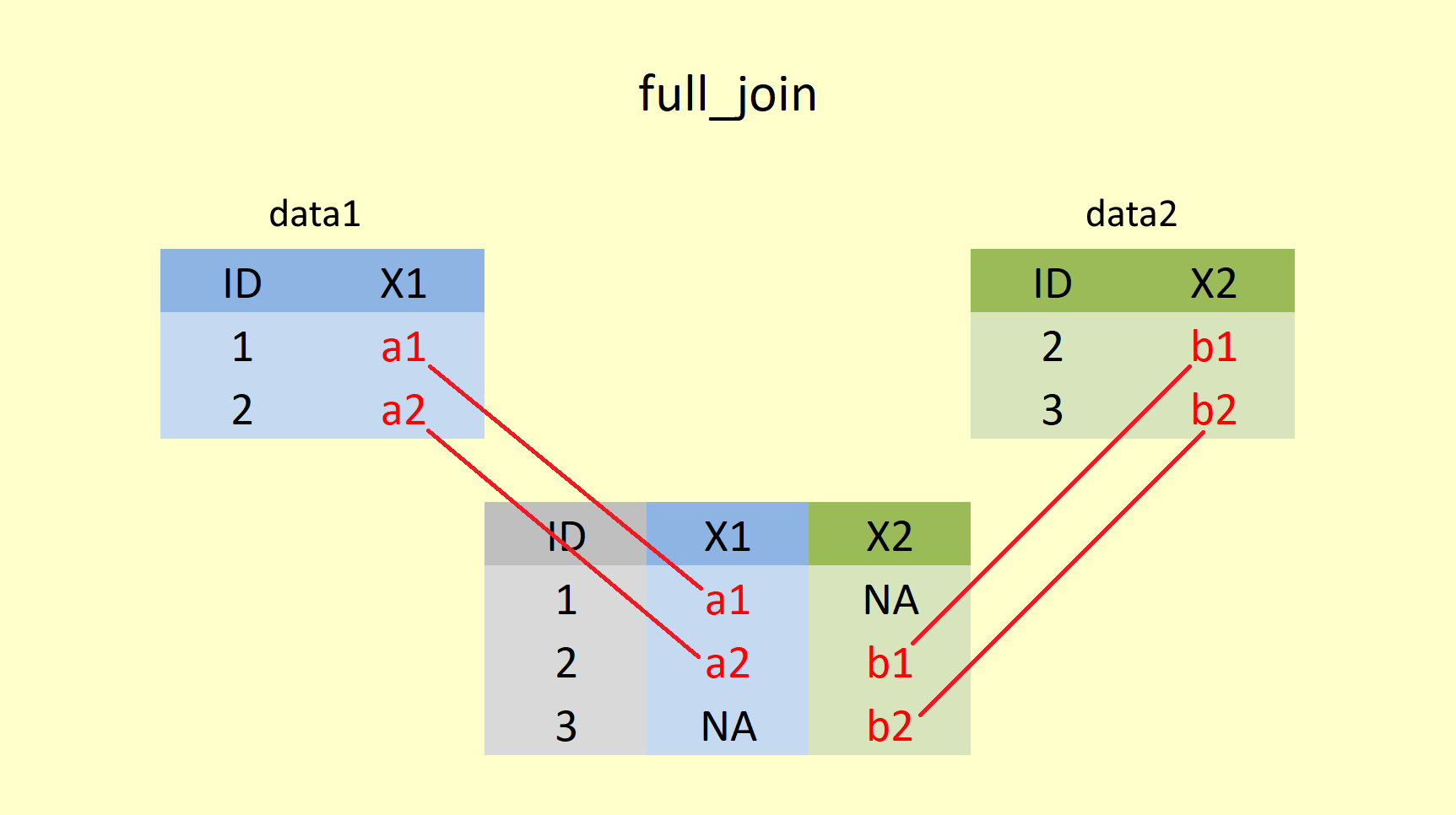
4.4.1.4 full_join()
A full join returns all rows and all columns from both x and y, whereby x is the first (left) table and y is the second (right) table. NA values fill unmatched rows.
full_join(data1, data2)## Joining, by = "ID"## # A tibble: 3 x 3
## ID X1 X2
## <int> <chr> <chr>
## 1 1 a1 <NA>
## 2 2 a2 b1
## 3 3 <NA> b2As you can see, ID values (1,2, and 3) from both dataframes are retained. ID = 3 does not exist in data1, and ID = 1 does not exist in data2, X1 and X2 are filled with NA respectively. Since the full join is the combination of both left join and right join, it would contain all student names, regardless of whether students dropped the course or not, and all student grades regardless of whether students sat the exam or not. Thus, it can be used to tailor student support and guidance and measure the difficulty level of the exam.
Question Time
Your turn
combine short_MH and extra_MH using full_join(). Save your results in the Global Environment as an object called MH_full. How many rows and columns are you expecting for MH_right?
MH_full <- full_join(short_MH, extra_MH, by = "ID")
glimpse(MH_full)
## Observations: 268
## Variables: 17
## $ ID <dbl> 1, 2, 3, 4, 5, 6, 7, 8, 9, 10, 11, 12, 13, 14, 15, 16, 1...
## $ inter_dom <chr> "Inter", "Inter", "Inter", "Inter", "Inter", "Inter", "I...
## $ Gender <chr> "Male", "Male", "Male", "Female", "Female", "Male", "Mal...
## $ Academic <chr> "Grad", "Grad", "Grad", "Grad", "Grad", "Grad", "Grad", ...
## $ Age <dbl> 24, 28, 25, 29, 28, 24, 23, 30, 25, 31, 28, 31, 29, 23, ...
## $ ToDep <dbl> 0, 2, 2, 3, 3, 6, 3, 9, 7, 3, 5, 8, 1, 3, 9, 6, 3, 3, 7,...
## $ ToSC <dbl> 34, 48, 41, 37, 37, 38, 46, 41, 36, 48, 32, 47, 48, 32, ...
## $ APD <dbl> 23, 8, 13, 16, 15, 18, 17, 16, 22, 8, 24, 17, 8, 9, 23, ...
## $ AHome <dbl> 9, 7, 4, 10, 12, 8, 6, 20, 12, 4, 8, 12, 11, 8, 16, 9, 1...
## $ APH <dbl> 11, 5, 7, 10, 5, 10, 10, 19, 13, 5, 10, 14, 5, 5, 15, 5,...
## $ Afear <dbl> 8, 4, 6, 8, 8, 8, 5, 15, 13, 12, 8, 13, 4, 4, 8, 4, 4, 4...
## $ ACS <dbl> 11, 3, 4, 6, 7, 7, 3, 11, 10, 3, 6, 9, 7, 6, 12, 13, 8, ...
## $ AGuilt <dbl> 2, 2, 3, 4, 4, 3, 2, 6, 6, 2, 6, 4, 2, 7, 8, 2, 5, 2, 2,...
## $ AMiscell <dbl> 27, 10, 14, 21, 31, 29, 15, 40, 33, 17, 30, 26, 17, 18, ...
## $ ToAS <dbl> 91, 39, 51, 75, 82, 83, 58, 127, 109, 51, 92, 95, 54, 57...
## $ GAD7 <dbl> 8, 1, NA, 0, 1, 14, 2, 1, 0, 2, 0, 2, 8, 0, 6, 12, 4, 0,...
## $ Employment <chr> "Unemployed", "Part", NA, "Part", "Full", "Unemployed", ...
We should receive 268 observations and 17 columns. All data is kept, including ID = 3, and GAD7 and Employment are filled up with NA values. In this case, full_join() produces the same output as left_join().
Hypothetical scenario
In the case of the student mental health data, we have seen that inner_join() and right_join() as well as left(join) and full_join() produce the same results. Can you think of a way how you would have to modify short_MH and/or extra_MH to produce different results for inner_join()/ right_join() or left(join)/full_join()?
Adding data for participant 269 to short_MH and 270 to extra_MH would do the trick:
-
inner_join()would still be the same output of 267 observations since the “overlapping”IDnumbers fordata1anddata2don’t change (1,2,4,5,…,268)
-
right_join()would prioritise the right tableextra_MH, leaving us withIDnumbers 1,2,4,5,…,268,270 (adding to a total of 268 observations. For ID = 270,X1would be filled withNA; ID = 3 would not be mentioned.
-
left(join)would prioritise the left tableshort_MH, selectingIDrows 1:269. For ID = 3 and ID = 269X2would showNA. ID = 270 would not be mentioned.
-
full_join()would add both datasets in full, showingIDvalues 1:270, with ID = 270 showingNAforX1, and ID = 3 and ID = 269 showingNAforX2.
All visualisation for the joins were adapted from https://statisticsglobe.com/r-dplyr-join-inner-left-right-full-semi-anti. The website also provides additional information on filtering joins (semi and anti joins) that we haven’t touched upon.
4.4.2 Binding Join Verbs
In contrast to mutating join verbs, binding join verbs simply combine tables without any need for matching. Dplyr provides bind_rows() and bind_cols() for combining tables by row and column respectively. When row binding, missing columns are replaced by NA values. When column binding, if the tables do not match by appropriate dimensions, an error will result.
Let’s take our simple example from above and see how data1 and data2 would be merged with bind_rows() and bind_cols().
bind_rows(data1, data2)## # A tibble: 4 x 3
## ID X1 X2
## <int> <chr> <chr>
## 1 1 a1 <NA>
## 2 2 a2 <NA>
## 3 2 <NA> b1
## 4 3 <NA> b2bind_rows() takes data2 and puts it underneath data1. Notice that the binding does not “care” that we have now two rows representing ID = 2. Since X1 and X2 do not exist in data1 and data2 respectively, NA are added.
bind_cols(data1, data2)## # A tibble: 2 x 4
## ID X1 ID1 X2
## <int> <chr> <int> <chr>
## 1 1 a1 2 b1
## 2 2 a2 3 b2bind_cols() takes data2 and puts it right next to data1. Since the column name ID has already been taken, column 3 gets called ID1.
In the case when the dimension between the dataframes do not match, bind_rows() would still work, whereas bind_cols() would produce an error message.
data3 <- tibble(ID = 3:5,
                X3 = c("c1", "c2", "c3"))

bind_rows(data1, data2, data3)
## # A tibble: 7 x 4
## ID X1 X2 X3
## <int> <chr> <chr> <chr>
## 1 1 a1 <NA> <NA>
## 2 2 a2 <NA> <NA>
## 3 2 <NA> b1 <NA>
## 4 3 <NA> b2 <NA>
## 5 3 <NA> <NA> c1
## 6 4 <NA> <NA> c2
## 7 5 <NA> <NA> c3bind_cols(data1, data3)
By the way, you can merge as many data objects as you like with the binding functions, whereas in the join functions, you are limited to two. However, you could use a pipe to combine the merged dataframe with a third.
example 1: bind_rows(data1, data2, data3)
example 2: full_join(data1, data2) %>% full_join(data3)
Your turn
You have finally found the missing data corresponding to ID number 3. This subject has a GAD7 score of 4 and is employed part-time. Store this information in a tibble called new_participant and bind it to the extra_MH dataset using bind_rows(). Store this merged output to your Global Environment as a new object called extra_MH_final.
new_participant <- tibble(ID = 3,
                          GAD7 = 4,
                          Employment = "Part")
extra_MH_final <- bind_rows(new_participant, extra_MH)
Follow-up Question
The dataset extra_MH_final now contains the same number of observations (rows) as short_MH. Use bind_cols() to merge these two datasets together in a tibble called MH_final. How many rows and columns are you expecting for MH_final to have and why?
Rows (or observations):
Columns (or variables):
MH_final <- bind_cols(short_MH, extra_MH_final)
We were expecting 268 observations (as both datasets have 268 rows) and 18 columns (i.e. 15 from short_MH and 3 from extra_MH_final). Notice that the ID column has been duplicated with an added suffix.
Follow-up Question 2
Using your knowledge of one-table verbs, exclude the column ID1, overwriting the object MH_final.
MH_final <- select(MH_final, -ID1)Follow-up Question 3
Rather than using bind_cols() and select(), can you think of a different way how you could have merged short_MH and extra_MH_final?
# One solution:
MH_final <- full_join(short_MH, extra_MH_final)
## Joining, by = "ID"
Actually, any of the other joins would have worked as well, though right_join() would have sorted the column ID differently. Try it out!
4.5 Additional information
Garrick Aden-Buie created some amazing gganimation gif to illustrate how the joins work. Check it out! https://www.garrickadenbuie.com/project/tidyexplain/
4.6 Summative Homework
The second summative assignment is available on moodle now.
Good luck.
Check that your Rmd file knits into a html file before submitting. Upload your Rmd file (not the knitted html) to moodle.