Chapter 5 Data Transformation 3: Tidy Data

Intended Learning Outcomes

The whole purpose of the next two lecture is to tidy up dataframe and expose you to a bunch of useful functions that would make your daily life easier when dealing with your own data. By the end of today, you will know

How to rearrange data from long format into to wide format and vice versa
How to combine and separate columns

This lesson is led by Gaby Mahrholz.

5.1 Pre-steps

All the functions for tidying data are within tidyverse so we need to make sure to load it into the library. Today’s lecture will make use of built-in dataframes which means we do not have to load any data into our Global Environment for the minute.

library(tidyverse)

5.2 Tidy data

“Happy families are all alike; every unhappy family is unhappy in its own way.” – Leo Tolstoy

“Tidy datasets are all alike, but every messy dataset is messy in its own way.” – Hadley Wickham

In this chapter, you will learn a consistent way to organise your data in R. Hadley Wickham and Garrett Grolemund call this tidy data. In most cases, data does not come in a tidy format. Researchers spend most of their time getting the data into the shape it needs to be for a particular analysis. The tools we introduce you to this week and next should form the basics for data wrangling. The idea is that tidy datasets are easier to work with in the long run.

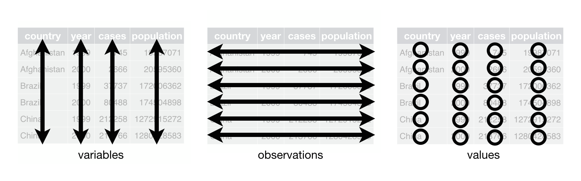
There are three interrelated rules which make a dataset tidy:

Each variable must have its own column.
Each observation must have its own row.
Each value must have its own cell.

If you want to know more about tidy data, Hadley Wickham’s paper can be found on https://vita.had.co.nz/papers/tidy-data.pdf or check out chapter 12 in the book R for Data Science (https://r4ds.had.co.nz/tidy-data.html).

5.3 gather() and spread()

gather() and spread() are part of tidyr (also part of the tidyverse package) and help you to rearrange the shape of your data. To get your data into long format, you would use gather(); if you wanted to get your data from long to wide format, you would need spread(). Here is a nice gif animation by Garrick Aden-Buie (https://www.garrickadenbuie.com/project/tidyexplain/#spread-and-gather) that shows you how gather() and spread() work.

5.3.1 gather()

We can start this lecture by looking at a practical example in the build-in dataset table1 to table5. They show the number of Tuberculosis cases documented by the World Health Organization in Afghanistan, Brazil, and China between 1999 and 2000 (the full dataset is called who). The data is part of the tidyverse package, so as long as we have tidyverse loaded into the library, there should not be an issue in accessing this dataset.

table1

## # A tibble: 6 x 4
##   country      year  cases population
##   <chr>       <int>  <int>      <int>
## 1 Afghanistan  1999    745   19987071
## 2 Afghanistan  2000   2666   20595360
## 3 Brazil       1999  37737  172006362
## 4 Brazil       2000  80488  174504898
## 5 China        1999 212258 1272915272
## 6 China        2000 213766 1280428583

table1 has a very tidy structure as it follows the three principles above - each variable is its own column, each observation is its own row, and each value is its own cell.

You can see the data contains values associated with four variables (country, year, cases, and population). table4a however, looks a touch not right.

table4a

## # A tibble: 3 x 3
##   country     `1999` `2000`
## * <chr>        <int>  <int>
## 1 Afghanistan    745   2666
## 2 Brazil       37737  80488
## 3 China       212258 213766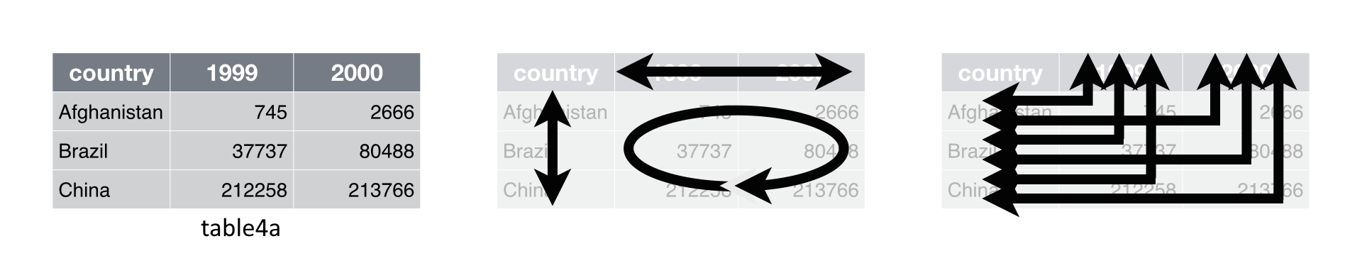

Somehow the values for the columns year and cases are missing and instead we find two separate columns for 1999 and 2000 that have all cases values listed. This is a problem as 1999 and 2000 are actual values and not variables. What we want to do, is gather 1999 and 2000 in one column year and respective values into a second column called cases.

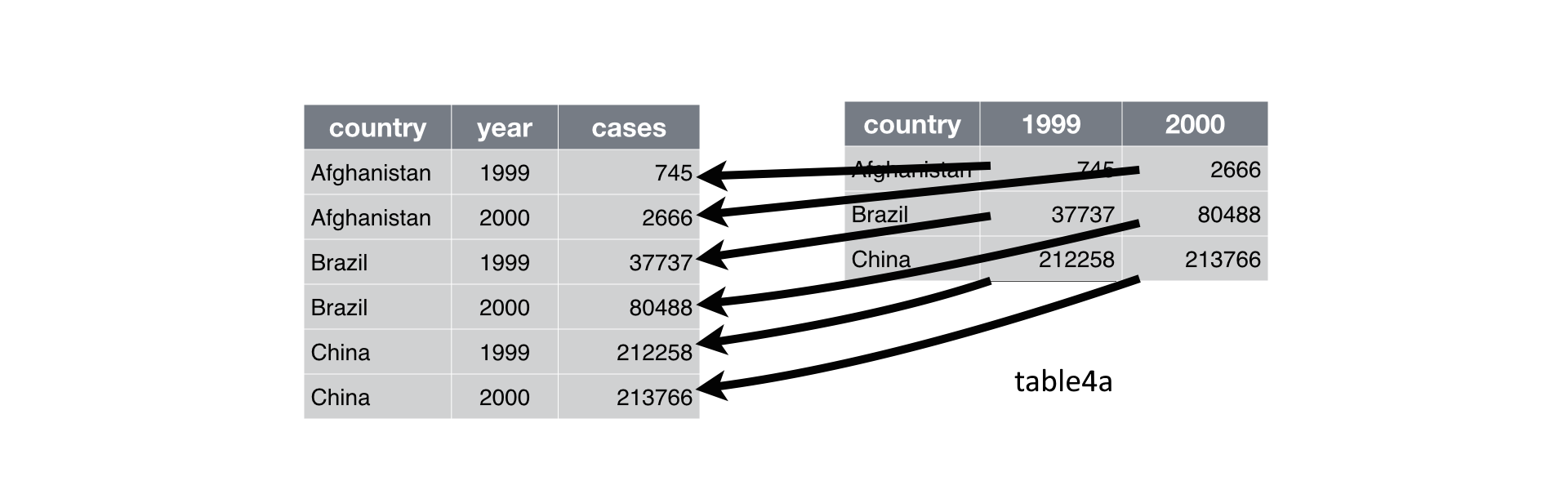
Currently the data is in what is called a wide format. The function gather() comes in handy when we want to get the data into the shape of a long format like in table1. gather() is structured like:

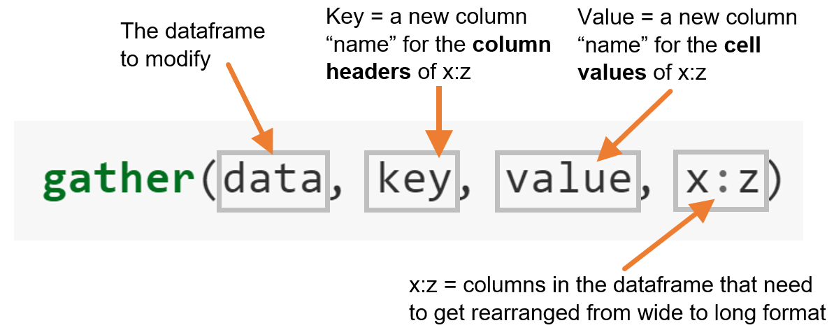
Let’s apply this formula to table4a

We need a dataframe that we want to modify -> table4a
We need to come up with the name of a new column in which the values of 1999 and 2000 will be stored -> year
We need to come up with the name of a new column in which all the case values will be stored -> cases
And finally, we need to tell R which columns in table4a we want to turn into long format (i.e. the columns of the 7 subscales) -> 1999 and 2000 (Note that “1999” and “2000” are non-syntactic names as they don’t start with a letter. The solution is to surround them in backticks.)

gather(table4a, key = year, value = cases, `1999`:`2000`)

## # A tibble: 6 x 3
##   country     year   cases
##   <chr>       <chr>  <int>
## 1 Afghanistan 1999     745
## 2 Brazil      1999   37737
## 3 China       1999  212258
## 4 Afghanistan 2000    2666
## 5 Brazil      2000   80488
## 6 China       2000  213766

Here we have only 2 columns to reshape 1999 and 2000. We could have written gather(table4a, year, cases, `1999`, `2000`).

Your turn

Look at table4b. There are two separate columns 1999 and 2000 with population values for Afghanistan, Brazil, and China. Use the gather() function on table4b to reshape it from wide format into long format.

gather(table4b, key = year, value = population, `1999`:`2000`)

## # A tibble: 6 x 3
##   country     year  population
##   <chr>       <chr>      <int>
## 1 Afghanistan 1999    19987071
## 2 Brazil      1999   172006362
## 3 China       1999  1272915272
## 4 Afghanistan 2000    20595360
## 5 Brazil      2000   174504898
## 6 China       2000  1280428583

5.3.2 spread()

Now onto the reverse. spread() will spread the data from long into wide format. When you have observations that are scattered across multiple rows, you can use spread() to split those rows up into separate variables. Let’s take a look at table2.

table2

## # A tibble: 12 x 4
##    country      year type            count
##    <chr>       <int> <chr>           <int>
##  1 Afghanistan  1999 cases             745
##  2 Afghanistan  1999 population   19987071
##  3 Afghanistan  2000 cases            2666
##  4 Afghanistan  2000 population   20595360
##  5 Brazil       1999 cases           37737
##  6 Brazil       1999 population  172006362
##  7 Brazil       2000 cases           80488
##  8 Brazil       2000 population  174504898
##  9 China        1999 cases          212258
## 10 China        1999 population 1272915272
## 11 China        2000 cases          213766
## 12 China        2000 population 1280428583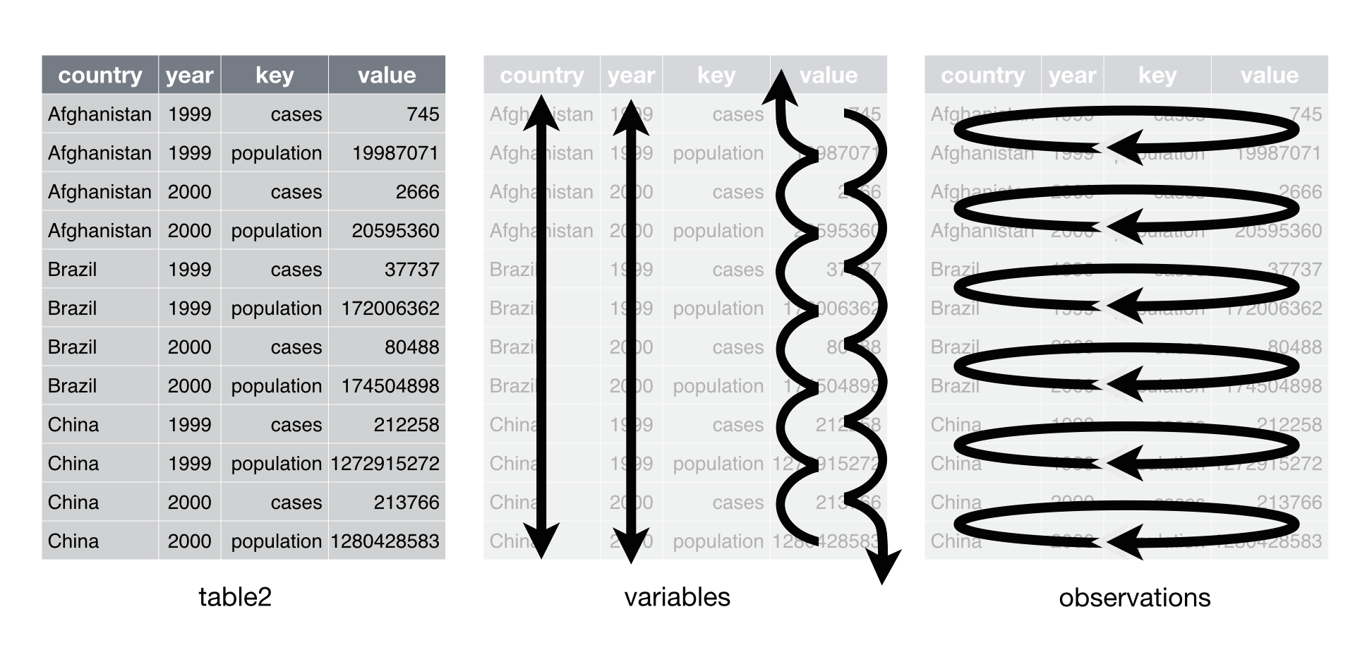

table2 has the variables cases and population stored in one column type and their respective values in count. However, cases and population are separate variables rather than values of type. So best to get them spread out into their own columns as shown in the image below.

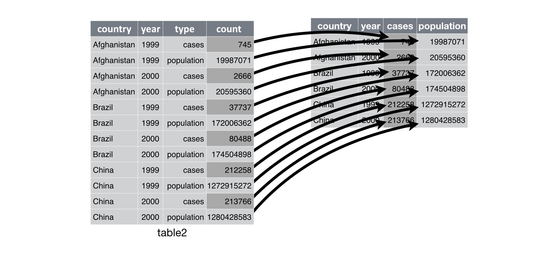
Take a look how spread() achieves that.

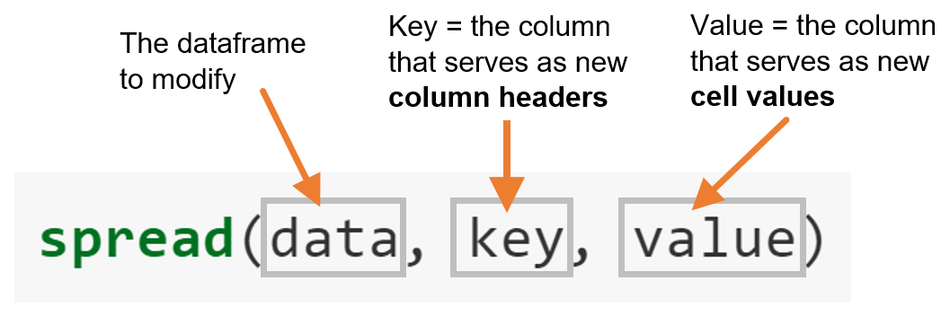
Let’s apply the formula above to table2:

We need a dataframe that we want to modify -> table2
We need to decide which of the columns in table2 will become the new column headers -> type
We need to decide which of the columns in table2 has all the data in it that will become the new cell values -> count

spread(table2, key = type, value = count)

## # A tibble: 6 x 4
##   country      year  cases population
##   <chr>       <int>  <int>      <int>
## 1 Afghanistan  1999    745   19987071
## 2 Afghanistan  2000   2666   20595360
## 3 Brazil       1999  37737  172006362
## 4 Brazil       2000  80488  174504898
## 5 China        1999 212258 1272915272
## 6 China        2000 213766 1280428583

Voila, cases and population are in their own columns.

Let me modify table1 a tiny bit.

table1_mod <- table1 %>% 
  mutate(percent = cases/ population * 100) %>% 
  gather(variable, values, cases:percent)

country	year	variable	values
Afghanistan	1999	cases	7.450000e+02
Afghanistan	2000	cases	2.666000e+03
Brazil	1999	cases	3.773700e+04
Brazil	2000	cases	8.048800e+04
China	1999	cases	2.122580e+05
China	2000	cases	2.137660e+05
Afghanistan	1999	population	1.998707e+07
Afghanistan	2000	population	2.059536e+07
Brazil	1999	population	1.720064e+08
Brazil	2000	population	1.745049e+08
China	1999	population	1.272915e+09
China	2000	population	1.280429e+09
Afghanistan	1999	percent	3.727400e-03
Afghanistan	2000	percent	1.294470e-02
Brazil	1999	percent	2.193930e-02
Brazil	2000	percent	4.612360e-02
China	1999	percent	1.667500e-02
China	2000	percent	1.669490e-02

Your turn

In the modified table above table1_mod, we added a percent column to see how much percentage of the population had Tuberculosis in 1999 and 2000 in each of the countries Afghanistan, Brazil, and China. But somehow, all numerical information has ended up in 1 column (values).

Your task is to spread the data back out, so that cases, population, and percentage values are in their own columns, titled as cases, population, and percent respectively. Store the new object in the Global Environment as table1_mod_corrected. When you are done, table1_mod_corrected should look like this…

country	year	cases	percent	population
Afghanistan	1999	745	0.0037274	19987071
Afghanistan	2000	2666	0.0129447	20595360
Brazil	1999	37737	0.0219393	172006362
Brazil	2000	80488	0.0461236	174504898
China	1999	212258	0.0166750	1272915272
China	2000	213766	0.0166949	1280428583

table1_mod_corrected <- spread(table1_mod, key = variable, value = values)

5.4 separate() and unite()

separate() turns a single character column into multiple columns, whereas unite() combines the values of multiple columns into one column.

5.4.1 separate()

Take a look at table3.

table3

## # A tibble: 6 x 3
##   country      year rate             
## * <chr>       <int> <chr>            
## 1 Afghanistan  1999 745/19987071     
## 2 Afghanistan  2000 2666/20595360    
## 3 Brazil       1999 37737/172006362  
## 4 Brazil       2000 80488/174504898  
## 5 China        1999 212258/1272915272
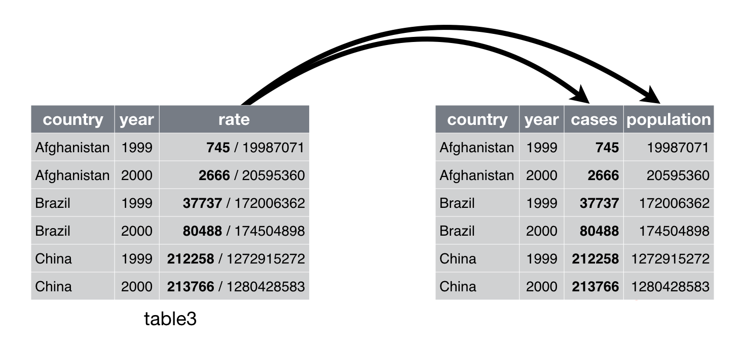
## 6 China        2000 213766/1280428583

In table3, two out of three principles of tidy data are violated. There are multiple values stored in column rate (rule 3) but these multiple values also belong to two different variables - cases and population respectively (rule 1).

Here, we would use separate() to split the column rate into two columns cases and population.

The function separate() is structured like this:

We would need

the data in which the column to separate is located -> table3,
the actual column we want to separate -> rate,
the into argument asking into how many columns we want to separate the old column and what we want to call these new columns -> c("cases", "population"), and
a separator argument -> "/".

separate(table3, rate, into = c("cases", "population"), sep = "/")

## # A tibble: 6 x 4
##   country      year cases  population
##   <chr>       <int> <chr>  <chr>     
## 1 Afghanistan  1999 745    19987071  
## 2 Afghanistan  2000 2666   20595360  
## 3 Brazil       1999 37737  172006362 
## 4 Brazil       2000 80488  174504898 
## 5 China        1999 212258 1272915272
## 6 China        2000 213766 1280428583

R has put all cell information before the / into a column we named cases, and everything after the / into the column we decided to call population. / will not appear in either column cases or population. The data is now in a tidy format.

By the way, the separator argument sep = can be any non-alphanumeric character, for example:

underscore (“_“),
comma (“,”),
semi-colon (“;”),
colon (“:”),
forward-slash (“/”),
space (" “) or
nothing (“”).

But watch out! When the separator is a full stop, you would need to add a double backward slash in front of it (sep = “\\.”).

5.4.2 additional arguments for separate()

5.4.2.1 Retaining the original column

If for some reason, you wanted to keep the original column, you can set an additional argument remove to FALSE.

separate(table3, rate, into = c("cases", "population"), sep = "/", remove = FALSE)

## # A tibble: 6 x 5
##   country      year rate              cases  population
##   <chr>       <int> <chr>             <chr>  <chr>     
## 1 Afghanistan  1999 745/19987071      745    19987071  
## 2 Afghanistan  2000 2666/20595360     2666   20595360  
## 3 Brazil       1999 37737/172006362   37737  172006362 
## 4 Brazil       2000 80488/174504898   80488  174504898 
## 5 China        1999 212258/1272915272 212258 1272915272
## 6 China        2000 213766/1280428583 213766 1280428583

5.4.2.2 Dropping parts of the original column

What if we were just interested retaining part of the data in the cell, for example keeping the column cases but not population. The solution would be to work with an NA argument. Defining the new columns as cases and NA will keep everything before the separator in the column cases, and drops everything after the separator.

separate(table3, rate, into = c("cases", NA), sep = "/")

## # A tibble: 6 x 3
##   country      year cases 
##   <chr>       <int> <chr> 
## 1 Afghanistan  1999 745   
## 2 Afghanistan  2000 2666  
## 3 Brazil       1999 37737 
## 4 Brazil       2000 80488 
## 5 China        1999 212258
## 6 China        2000 213766

Your turn

Separate the column rate in table3 to keep only the values after the separator in a column called population. Drop the values in front of the separator. Retain the column rate as well.

separate(table3, rate, into = c(NA, "population"), sep = "/", remove = FALSE)

## # A tibble: 6 x 4
##   country      year rate              population
##   <chr>       <int> <chr>             <chr>     
## 1 Afghanistan  1999 745/19987071      19987071  
## 2 Afghanistan  2000 2666/20595360     20595360  
## 3 Brazil       1999 37737/172006362   172006362 
## 4 Brazil       2000 80488/174504898   174504898 
## 5 China        1999 212258/1272915272 1272915272
## 6 China        2000 213766/1280428583 1280428583

5.4.2.3 Separating by position

It is also possible to separate by position. sep = 2 would split the column between the second and third character/ number etc.

Let’s try that the separation by position. We will keep 4 letters from each country name rather than the whole word, and drop the rest.

separate(table3, country, into = c("country", NA), sep = 4)

## # A tibble: 6 x 3
##   country  year rate             
##   <chr>   <int> <chr>            
## 1 Afgh     1999 745/19987071     
## 2 Afgh     2000 2666/20595360    
## 3 Braz     1999 37737/172006362  
## 4 Braz     2000 80488/174504898  
## 5 Chin     1999 212258/1272915272
## 6 Chin     2000 213766/1280428583

5.4.2.4 Separating into more than 2 columns

Special case. Let’s modify table3 a little bit by adding a new column with a value of 200 and unite that column with column rate.

table3_mod <- table3 %>% 
  mutate(new = 200) %>% 
  unite(rate, rate, new, sep = "/")

Now column rate has 3 sets of numbers, separated by two /. If we define we want to split the data into 2 columns, the first 2 sets of numbers are kept, and the third one is dropped with a warning. The code is still executed but the warning indicates that it might not have gone as planned. Hence, it is always good to check that the data object in the Global Environment looks exactly as what you have intended.

separate(table3_mod, rate, into = c("cases", "population"), sep = "/")

## Warning: Expected 2 pieces. Additional pieces discarded in 6 rows [1, 2, 3, 4,
## 5, 6].

## # A tibble: 6 x 4
##   country      year cases  population
##   <chr>       <int> <chr>  <chr>     
## 1 Afghanistan  1999 745    19987071  
## 2 Afghanistan  2000 2666   20595360  
## 3 Brazil       1999 37737  172006362 
## 4 Brazil       2000 80488  174504898 
## 5 China        1999 212258 1272915272
## 6 China        2000 213766 1280428583

If we are separating the columns and wanted to keep all sets of numbers, one in each column, we would use an into argument that includes 3 new columns.

separate(table3_mod, rate, into = c("cases", "population", "200"), sep = "/")

## # A tibble: 6 x 5
##   country      year cases  population `200`
##   <chr>       <int> <chr>  <chr>      <chr>
## 1 Afghanistan  1999 745    19987071   200  
## 2 Afghanistan  2000 2666   20595360   200  
## 3 Brazil       1999 37737  172006362  200  
## 4 Brazil       2000 80488  174504898  200  
## 5 China        1999 212258 1272915272 200  
## 6 China        2000 213766 1280428583 200

Technically, you would not need a separator argument in the case above, as separate() splits the data whenever it detects a non-alphanumeric character (i.e. a character that isn’t a number or letter). Saying that, the separator argument is needed when your column contains non-alphanumeric characters as part of your cell values.

If the values in population and 200 (separated by a /) were some sort of ID_code, AND we wanted to split the data into 2 columns, after the first / only, we would have to include an extra argument, and set it to "merge".

separate(table3_mod, rate, into = c("cases", "ID_code"), sep = "/", extra = "merge")

## # A tibble: 6 x 4
##   country      year cases  ID_code       
##   <chr>       <int> <chr>  <chr>         
## 1 Afghanistan  1999 745    19987071/200  
## 2 Afghanistan  2000 2666   20595360/200  
## 3 Brazil       1999 37737  172006362/200 
## 4 Brazil       2000 80488  174504898/200 
## 5 China        1999 212258 1272915272/200
## 6 China        2000 213766 1280428583/200

There is still a tiny bit off in the tb_cases. Can you spot what it is? * Hint: Think about if you wanted to sum up all the TB cases occurred in the 3 countries within the years 1999, and 2000.

The new columns ID_code and cases are character columns. Whilst this is fine for ID_code, it is less beneficial for cases. If we wanted to sum up the cases column, values would need to be numerical. We could use the converting function as.integer().

table3_mod %>% 
  separate(rate, into = c("cases", "ID_code"), sep = "/", extra = "merge") %>% 
  mutate(cases = as.integer(cases))

## # A tibble: 6 x 4
##   country      year  cases ID_code       
##   <chr>       <int>  <int> <chr>         
## 1 Afghanistan  1999    745 19987071/200  
## 2 Afghanistan  2000   2666 20595360/200  
## 3 Brazil       1999  37737 172006362/200 
## 4 Brazil       2000  80488 174504898/200 
## 5 China        1999 212258 1272915272/200
## 6 China        2000 213766 1280428583/200

5.4.2.5 Converting data types

The slightly quicker and perhaps more elegant solution would be to add another argument convert to separate() and set it to TRUE. This will convert cases to integer and leave ID_code as character due to the non-numerical /.

table3_mod %>% 
  separate(rate, into = c("cases", "ID_code"), sep = "/", extra = "merge", convert = TRUE)

## # A tibble: 6 x 4
##   country      year  cases ID_code       
##   <chr>       <int>  <int> <chr>         
## 1 Afghanistan  1999    745 19987071/200  
## 2 Afghanistan  2000   2666 20595360/200  
## 3 Brazil       1999  37737 172006362/200 
## 4 Brazil       2000  80488 174504898/200 
## 5 China        1999 212258 1272915272/200
## 6 China        2000 213766 1280428583/200

5.4.3 unite()

Take a look at table5.

table5

## # A tibble: 6 x 4
##   country     century year  rate             
## * <chr>       <chr>   <chr> <chr>            
## 1 Afghanistan 19      99    745/19987071     
## 2 Afghanistan 20      00    2666/20595360    
## 3 Brazil      19      99    37737/172006362  
## 4 Brazil      20      00    80488/174504898  
## 5 China       19      99    212258/1272915272
## 6 China       20      00    213766/1280428583

Here the values in column year are split into century and year which is not very useful. Best to merge the 2 columns together as shown in the image below.

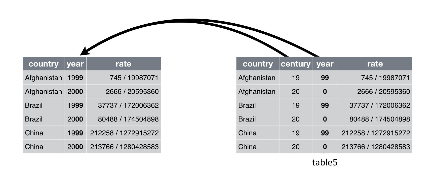
unite() (the inverse of separate) can help to combine the values of century and year into a single column. It is used less frequently than it’s counterpart, but is still a useful function to know.

The function unite() is structured like this:

We would need the data table5, a new column we want to create year, the two columns we would like to combine (century and year), and define the separator as “nothing” since the default is sep = “_“.

unite(table5, year, century, year, sep = "")

## # A tibble: 6 x 3
##   country     year  rate             
##   <chr>       <chr> <chr>            
## 1 Afghanistan 1999  745/19987071     
## 2 Afghanistan 2000  2666/20595360    
## 3 Brazil      1999  37737/172006362  
## 4 Brazil      2000  80488/174504898  
## 5 China       1999  212258/1272915272
## 6 China       2000  213766/1280428583

Yay! The data of table5 is in a tidier format now - at least for column year. Ah, but we didn’t save the changes as an object in our Global Environment.

Your turn

Let’s combine the two steps of tidying table5 in a single pipe %>% - separate the rate column into cases and population, and unite the columns year and century into a new column year. Store the new object as tb_cases in the Global Environment. Make sure, the columns cases and population are integer values.

tb_cases <- table5 %>% 
  separate(rate, into = c("cases", "population"), sep = "/", convert = TRUE) %>% 
  unite(year, century, year, sep = "")
tb_cases

## # A tibble: 6 x 4
##   country     year   cases population
##   <chr>       <chr>  <int>      <int>
## 1 Afghanistan 1999     745   19987071
## 2 Afghanistan 2000    2666   20595360
## 3 Brazil      1999   37737  172006362
## 4 Brazil      2000   80488  174504898
## 5 China       1999  212258 1272915272
## 6 China       2000  213766 1280428583

The year column is still a character column. In this case, it does not matter too much, as 1999 and 2000 are levels of the column year and very unlikely to be involved in any calculations. In case we are dealing with actual numerical value and have the need to convert the data type, we need to use the function as.integer() as unite does not have a convert argument available.

tb_cases_converted <- tb_cases %>% 
  mutate(year = as.integer(year))
tb_cases_converted

## # A tibble: 6 x 4
##   country      year  cases population
##   <chr>       <int>  <int>      <int>
## 1 Afghanistan  1999    745   19987071
## 2 Afghanistan  2000   2666   20595360
## 3 Brazil       1999  37737  172006362
## 4 Brazil       2000  80488  174504898
## 5 China        1999 212258 1272915272
## 6 China        2000 213766 1280428583

5.4.4 additional arguments for unite()

5.4.4.1 Retaining the original column

Similarly to separate(), unite also comes with a remove statement, so if you wanted to keep the original columns before merging them together, you would code

unite(table5, year_combined, century, year, sep = "", remove = FALSE)

## # A tibble: 6 x 5
##   country     year_combined century year  rate             
##   <chr>       <chr>         <chr>   <chr> <chr>            
## 1 Afghanistan 1999          19      99    745/19987071     
## 2 Afghanistan 2000          20      00    2666/20595360    
## 3 Brazil      1999          19      99    37737/172006362  
## 4 Brazil      2000          20      00    80488/174504898  
## 5 China       1999          19      99    212258/1272915272
## 6 China       2000          20      00    213766/1280428583

5.4.4.2 Removing missing values before uniting columns

unite() also comes with an na.rm statement that will remove missing values prior to uniting the values of a column (actually, the values have to be a “character” column). Let me modify table5 a wee bit to make that point.

table5_mod <- table5 %>% 
  mutate(new = rep(c("200", NA), 3))

table5_mod

## # A tibble: 6 x 5
##   country     century year  rate              new  
##   <chr>       <chr>   <chr> <chr>             <chr>
## 1 Afghanistan 19      99    745/19987071      200  
## 2 Afghanistan 20      00    2666/20595360     <NA> 
## 3 Brazil      19      99    37737/172006362   200  
## 4 Brazil      20      00    80488/174504898   <NA> 
## 5 China       19      99    212258/1272915272 200  
## 6 China       20      00    213766/1280428583 <NA>

If we wanted to combine the values of rate and new, we would code

unite(table5_mod, rate, rate, new, sep = "/")

## # A tibble: 6 x 4
##   country     century year  rate                 
##   <chr>       <chr>   <chr> <chr>                
## 1 Afghanistan 19      99    745/19987071/200     
## 2 Afghanistan 20      00    2666/20595360/NA     
## 3 Brazil      19      99    37737/172006362/200  
## 4 Brazil      20      00    80488/174504898/NA   
## 5 China       19      99    212258/1272915272/200
## 6 China       20      00    213766/1280428583/NA

See how R adds the missing values onto rate, which we do not want. To avoid that happening, we can use the na.rm statement which removes missing values in columns of data type character before merging the columns.

unite(table5_mod, rate, rate, new, sep = "/", na.rm = TRUE)

## # A tibble: 6 x 4
##   country     century year  rate                 
##   <chr>       <chr>   <chr> <chr>                
## 1 Afghanistan 19      99    745/19987071/200     
## 2 Afghanistan 20      00    2666/20595360        
## 3 Brazil      19      99    37737/172006362/200  
## 4 Brazil      20      00    80488/174504898      
## 5 China       19      99    212258/1272915272/200
## 6 China       20      00    213766/1280428583

5.5 Bonus materials: mutate row names from the mtcars

Remember, in lecture 2 when we were talking about the mtcars dataset and how the car types were not in listed as a separate column but rather row names? Let’s just read in the data and have another quick look to jog our memories…

df_mtcars <- mtcars

head(df_mtcars)

##                    mpg cyl disp  hp drat    wt  qsec vs am gear carb
## Mazda RX4         21.0   6  160 110 3.90 2.620 16.46  0  1    4    4
## Mazda RX4 Wag     21.0   6  160 110 3.90 2.875 17.02  0  1    4    4
## Datsun 710        22.8   4  108  93 3.85 2.320 18.61  1  1    4    1
## Hornet 4 Drive    21.4   6  258 110 3.08 3.215 19.44  1  0    3    1
## Hornet Sportabout 18.7   8  360 175 3.15 3.440 17.02  0  0    3    2
## Valiant           18.1   6  225 105 2.76 3.460 20.22  1  0    3    1

You can see much better what I’m talking about when you view your df_mtcars.

Now, that we have learnt about the mutate() function, we can attempt to get all of these row names into a new column. All we have to do is combining a function called rownames() with mutate(). We also could use some more of these handy pipes %>% you learnt about last week.

df_mtcars <- mtcars %>% 
  mutate(Car_type = rownames(mtcars))

In this example, we have taken the dataset mtcars, then added a new column called Car_type with mutate(). The column Car_type should then hold all the values that were previously listed as the row names in the original mtcars data.

head(df_mtcars)

##    mpg cyl disp  hp drat    wt  qsec vs am gear carb          Car_type
## 1 21.0   6  160 110 3.90 2.620 16.46  0  1    4    4         Mazda RX4
## 2 21.0   6  160 110 3.90 2.875 17.02  0  1    4    4     Mazda RX4 Wag
## 3 22.8   4  108  93 3.85 2.320 18.61  1  1    4    1        Datsun 710
## 4 21.4   6  258 110 3.08 3.215 19.44  1  0    3    1    Hornet 4 Drive
## 5 18.7   8  360 175 3.15 3.440 17.02  0  0    3    2 Hornet Sportabout
## 6 18.1   6  225 105 2.76 3.460 20.22  1  0    3    1           Valiant

We can now look at the data df_mtcars, and see that the new column was added at the end of the dataset. What would we have to do to make Car_type the first column in the dataframe?

# We could use the fuction select()
df_mtcars <- mtcars %>% 
  mutate(Car_type = rownames(mtcars)) %>% 
  select(Car_type, mpg:carb)

head(df_mtcars)

##            Car_type  mpg cyl disp  hp drat    wt  qsec vs am gear carb
## 1         Mazda RX4 21.0   6  160 110 3.90 2.620 16.46  0  1    4    4
## 2     Mazda RX4 Wag 21.0   6  160 110 3.90 2.875 17.02  0  1    4    4
## 3        Datsun 710 22.8   4  108  93 3.85 2.320 18.61  1  1    4    1
## 4    Hornet 4 Drive 21.4   6  258 110 3.08 3.215 19.44  1  0    3    1
## 5 Hornet Sportabout 18.7   8  360 175 3.15 3.440 17.02  0  0    3    2
## 6           Valiant 18.1   6  225 105 2.76 3.460 20.22  1  0    3    1

5.6 Additional information

More information on stuff we covered today and beyond can be found here:

https://r4ds.had.co.nz “R 4 Data Science” by Garrett Grolemund and Hadley Wickham is the official guidebook for R
https://suzan.rbind.io/categories/tutorial/ She has some pretty cool tutorials on data wrangling

5.7 Formative Homework

The formative assessment can now be downloaded from moodle. There is no need to submit your answers to moodle.