Chapter 4 Data Transformation 2: More One and Two Table Verbs
Intended Learning Outcomes
- Become comfortable with the Wickham Six dplyr one-table verbs:
select()arrange()filter()mutate()group_by()summarise()
Be able to chain functions together using the pipe operator (
%>%)Be able to use the following dplyr two-table verbs:
- Mutating joins:
left_join(),right_join(),full_join(),inner_join() - Binding joins:
bind_rows(),bind_cols()
This lesson is led by Jaimie Torrance.
4.1 Pre-Steps
- Make sure to download todays materials and save them to your desired working directory. Make sure you have all the correct files including the
L4_Stubfile, and the data files;CareerStats2.csv,wos_seasonal_sun.csv,wos_seasonal_rain.csv,wos_monthly_sun.csvandwos_monthly_rain.csv. - Open the
L4_stubfile. - Load
tidyverseinto the library. - Read the data from
CareerStats2.csvinto yourGlobal EnvironmentasMMA_Data.
library(tidyverse)
MMA_Data <- read_csv("CareerStats2.csv")
4.2 Practicing the Wikham Six
The first part of todays class will be practicing the Wickham Six some more, as was mentioned before, the vast majority of your "data time" will be wrangling your data, and most of that can be done with these six functions, so it's good to practice with them. First you'll see an example of each function to refresh your memory. Then you will be asked to try for yourself, these will be a little more involved than last week to really test you. If you are stuggling you can check the solutions, but try yourself first, and answer the questions too, this will help you check your code is correct.
4.2.1 select()
First up lets try to narrow down this big data set, by taking MMA_Data, and selecting only the variables; ID, Height, Weight, BMI, Reach and Stance. We will store this in Example_1.
Example_1 <- select(MMA_Data, ID, Height, Weight:Reach, Stance)
Example_1
## # A tibble: 199 x 6
## ID Height Weight BMI Reach Stance
## <chr> <dbl> <dbl> <dbl> <dbl> <chr>
## 1 056c493bbd76a918 64 125 21.5 64 Orthodox
## 2 b102c26727306ab6 65 125 20.8 67 Orthodox
## 3 80eacd4da0617c57 64 125 21.5 65 Southpaw
## 4 a4de54ea806fb525 64 125 21.5 63 Orthodox
## 5 aa72b0f831d0bfe5 65 125 20.8 68 Orthodox
## 6 92437c6775b3f7d1 66 125 20.2 66 Orthodox
## 7 5aedf14771ca82d2 64 125 21.5 65 Southpaw
## 8 a0f0004aadf10b71 65 125 20.8 67 Orthodox
## 9 f53c1f4ceeed8c08 65 125 20.8 65 Orthodox
## 10 ab2b4ff41d6ebe0f 66 125 20.2 65 Orthodox
## # ... with 189 more rows
Notice, this could also have been written as follows; Example_1 <- select(MMA_Data, ID, Height, Weight, BMI, Reach, Stance)
We can use the : operator to sequence together columns that are next to each other in the original dataframe, this can save time but it is not necessary.
Question Time
Your turn
Using select() keep everything from Example_1 but except Reach, and store this in an object names Q1.
# Jaimie's solutions
Q1 <- select(Example_1, -Reach)
#OR
Q1 <- select(Example_1, ID, Height, Weight, BMI, Stance)
4.2.2 arrange()
Lets move on to arrange(); lets take the table Example_1, and arrange it first by Weight, then by BMI, we'll store this in Example_2.
Example_2 <- arrange(Example_1, Weight, BMI)
Example_2
## # A tibble: 199 x 6
## ID Height Weight BMI Reach Stance
## <chr> <dbl> <dbl> <dbl> <dbl> <chr>
## 1 199eb7cf6ae90294 69 125 18.5 71 Orthodox
## 2 0fd5f4b838e890cc 68 125 19.0 70 Orthodox
## 3 67c1d46f4ed16f9e 68 125 19.0 70 Orthodox
## 4 792be9a24df82ed6 67 125 19.6 70 Orthodox
## 5 92437c6775b3f7d1 66 125 20.2 66 Orthodox
## 6 ab2b4ff41d6ebe0f 66 125 20.2 65 Orthodox
## 7 a0c64f272b65d441 66 125 20.2 68 Orthodox
## 8 1a31ef98efce7a79 66 125 20.2 66 Switch
## 9 2fe9032955c2e013 66 125 20.2 69 Switch
## 10 b102c26727306ab6 65 125 20.8 67 Orthodox
## # ... with 189 more rowsQuestion Time
What is the height of the top entry in Example_2?
Your turn
Using arrange(), take the table Example_1 and arrange it first by Reach in desceding order, then by Height in ascending order. Store the result in Q2.
# Jaimie's solution
Q2 <- arrange(Example_1, desc(Reach), desc(Height))
What is the BMI of the top entry in Q2?
4.2.3 filter()
Now onto filter() which has so many uses! Lets filter out all the athletes who are over 31 years of age
Example_3 <- filter(MMA_Data, Age <=31)
Example_3
## # A tibble: 97 x 32
## ID Age Height HeightClass Weight BMI Reach ReachClass Stance
## <chr> <dbl> <dbl> <chr> <dbl> <dbl> <dbl> <chr> <chr>
## 1 a4de~ 25.4 64 Short 125 21.5 63 Below Ortho~
## 2 a0f0~ 28.7 65 Short 125 20.8 67 Below Ortho~
## 3 f53c~ 30 65 Short 125 20.8 65 Below Ortho~
## 4 ab2b~ 26.8 66 Average 125 20.2 65 Below Ortho~
## 5 87f1~ 30.4 65 Short 125 20.8 65 Below Ortho~
## 6 0fd5~ 26.7 68 Average 125 19.0 70 Below Ortho~
## 7 2099~ 29.3 65 Short 125 20.8 68 Below Ortho~
## 8 a0c6~ 27.9 66 Average 125 20.2 68 Below Ortho~
## 9 67c1~ 29.0 68 Average 125 19.0 70 Below Ortho~
## 10 792b~ 25.0 67 Average 125 19.6 70 Below Ortho~
## # ... with 87 more rows, and 23 more variables: WeightClass <chr>,
## # T_Wins <dbl>, T_Losses <dbl>, T_Fights <dbl>, Success <dbl>,
## # W_by_Decision <dbl>, `W_by_KO/TKO` <dbl>, W_by_Sub <dbl>,
## # L_by_Decision <dbl>, `L_by_KO/TKO` <dbl>, L_by_Sub <dbl>, PWDec <dbl>,
## # PWTko <dbl>, PWSub <dbl>, PLDec <dbl>, PLTko <dbl>, PLSub <dbl>,
## # Available <dbl>, TTime <dbl>, Time_Avg <dbl>, TLpM <dbl>, AbpM <dbl>,
## # SubAtt_Avg <dbl>Question Time
How many athletes (observations) are left in Example_3?
Your turn
Using filter(), take the original table MMA_Data and keep only those athletes in the 'Flyweight' and 'Lightweight' WeightClasses Store the result in Q3.
# Jaimie's solution
Q3 <- filter(MMA_Data, WeightClass %in% c("Flyweight", "Lightweight"))
How many athletes (observations) are left in Q3?
Your turn
Now try taking the original table MMA_Data and keep only those athletes from the "Welterweight" WeightClass, who are over 72 inches in Height. Store the result in Q4. - Hint - remember they will need to match both conditions
# Jaimie's solution
Q4 <- filter(MMA_Data, WeightClass == "Welterweight", Height <= 72)
How many athletes (observations) are left in Q4?
Your turn
Now try taking the original table MMA_Data and keep only those athletes who have the "Orthodox" Stance AND have 27 or more total fights (T_Fights) OR 15 or more wins by submission (W_by_Sub). Store the result in Q5. - Hint - No matter what they need to have the Orthodox stance, regardless of the other conditions
# Jaimie's solution
Q5 <- filter(MMA_Data, Stance == "Orthodox" & (T_Fights >= 27 | W_by_Sub >= 15))
#OR
Q5 <- filter(MMA_Data, Stance == "Orthodox", (T_Fights >= 27 | W_by_Sub >= 15))There is essentially 2 parts to this question; the first criteria is to find athletes who have the "orthodox" stance... that's the first requirement... then if they matched that criteria, we want to check, if they have EITHER 27 or more total fights OR 15 or more wins by submission, which is why we need to put the second "either/or" criteria in brackets, so R knows to treat them together.
If you take the brackets out, it will treat the first two criteria as a joint criteria and the | "Or" operator creates the break. Meaning R thinks you are asking for; Athletes with the orthodox stance and 27 or more total fights... OR athletes with 15 or more wins by submission. Try running the code without the brackets and seeing what happens
Q5Alt <- filter(MMA_Data, Stance == "Orthodox" & T_Fights >= 27 | W_by_Sub >= 15)
Hopefully now you can understand the difference.
How many athletes (observations) are left in Q5?
4.2.4 mutate()
Moving on to mutate() now.
Lets add a new column onto the table Example_1, that shows Reach but in meters rather than inches, and we'll call it ReachM. We can make this column with mutate() by converting the inches value in the original Reach column into centimeters, by multiplying (*) the value by 2.54 and then dividing (/) the result by 100.
Example_4 <- mutate(Example_1, ReachM = (Reach*2.54)/100)
Example_4
## # A tibble: 199 x 7
## ID Height Weight BMI Reach Stance ReachM
## <chr> <dbl> <dbl> <dbl> <dbl> <chr> <dbl>
## 1 056c493bbd76a918 64 125 21.5 64 Orthodox 1.63
## 2 b102c26727306ab6 65 125 20.8 67 Orthodox 1.70
## 3 80eacd4da0617c57 64 125 21.5 65 Southpaw 1.65
## 4 a4de54ea806fb525 64 125 21.5 63 Orthodox 1.60
## 5 aa72b0f831d0bfe5 65 125 20.8 68 Orthodox 1.73
## 6 92437c6775b3f7d1 66 125 20.2 66 Orthodox 1.68
## 7 5aedf14771ca82d2 64 125 21.5 65 Southpaw 1.65
## 8 a0f0004aadf10b71 65 125 20.8 67 Orthodox 1.70
## 9 f53c1f4ceeed8c08 65 125 20.8 65 Orthodox 1.65
## 10 ab2b4ff41d6ebe0f 66 125 20.2 65 Orthodox 1.65
## # ... with 189 more rowsQuestion Time
Your turn
Take the table Example_1 and mutate a new column onto it called BMI_Alt, this time attempting to recalculate BMI using the Weight and Height variables. The calculation for BMI is; weight in kilograms devided by height in meters squared. Lets break down the steps, you will need to; - multiply Weight by 0.453 (to convert lbs to kgs) - divide that by... - Height multiplied 2.54 (to convert inches to cm), which you divide by 100 (to convert to m), which you then square Store the result in Q5.
-
Hint - the
^symbol is for calculating "to the power of"
# Jaimie's solution
Q6 <- mutate(Example_1, BMI_Alt = (Weight*0.453)/(((Height*2.54)/100)^2))
Don't be worried if your new column is different by a few decimals (the original BMI was created with a slightly different calculation with different rounding). If they look approximately similar you have done it correctly.
4.2.5 group_by() and summarise()
Now let's brush up on group_by and summarise().
Here we will take the original table MMA_Data and group that data by WeightClass. Then we will create mean() summary stats for: Number of hits landed per minute (TLpM) and we'll call that column MeanHit, Number of hits absorbed per minute (AbpM) and we'll call that column MeanAbsorb, And average fight length (Time_Avg) and we'll call that column MeanTime.
Example_5a <- group_by(MMA_Data, WeightClass)
Example_5b <- summarise(Example_5a, MeanHit = mean(TLpM), MeanAbsorb = mean(AbpM), MeanTime = mean(Time_Avg))
## `summarise()` ungrouping output (override with `.groups` argument)Example_5b## # A tibble: 8 x 4
## WeightClass MeanHit MeanAbsorb MeanTime
## <chr> <dbl> <dbl> <dbl>
## 1 Bantamweight 5.46 3.38 11.3
## 2 Featherweight 5.43 3.46 11.8
## 3 Flyweight 4.78 2.64 11.9
## 4 Heavyweight 5.28 3.14 10.1
## 5 LightHeavyweight 6.05 2.97 9.12
## 6 Lightweight 5.19 3.25 9.93
## 7 Middleweight 5.11 2.78 10.2
## 8 Welterweight 5.09 2.94 11.7Question Time
Which weightclass has the highest Hit average?
Which weightclass has the lowest Absorbtion average?
Which weightclass has the highest average time?
Your turn
Take the original table MMA_Data and group that data by Stance and HeightClass and store that in Q7a. Then create summary stats for success rate (Success), you should have columns called; MedSuccess that shows the median success rate MaxSuccess that shows the maximum success rate MinSuccess that shows the minimum success rate SDSuccess that shows the standard deviation of success rate The resulting table should be stored in Q7b.
# Jaimie's solution
Q7a <- group_by(MMA_Data, Stance, HeightClass)
Q7b <- summarise(Q7a, MedSuccess = median(Success), MaxSuccess = max(Success), MinSuccess = min(Success), SDSuccess = sd(Success))
## `summarise()` regrouping output by 'Stance' (override with `.groups` argument)Which Stance/HeightClass combo has the highest median success rate? (enter your answers in the format Stance/HeightClass)
What is the minimum success rate of tall athletes with an orthodox stance?
What is the standard deviation in success rate for short athletes with a southpaw stance? (write your answer to 3 decimal places)
4.2.6 Bringing it all together
Question Time
Your turn This is another multi-part question...
-
Take the original table
MMA_Data, and select justID,WeightClass,Stance,T_Wins,W_by_Decision,W_by_KO/TKOandW_by_Sub. Store the result inQ8a. -
Take
Q8aand filter out all the athletes with the "Southpaw"Stance. Store the result in Q8b. -
Take
Q8band mutate on a new column calledPerc_W_by_Decthat shows the percentage of total wins (T_Wins) that are accounted for by decisions (W_by_Decision). Store the result inQ8c. -
Take
Q8cand group that data byWeightClass. Store the result inQ8d. -
Take
Q8dand create summary stats that show the mean ofPerc_W_by_Dec. Store the result inQ8e.
# Jaimie's solution
Q8a <- select(MMA_Data, ID, WeightClass, Stance, T_Wins, W_by_Decision, "W_by_KO/TKO", W_by_Sub)
Q8b <- filter(Q8a, Stance != "Southpaw")
Q8c <- mutate(Q8b, Perc_W_by_Dec = (W_by_Decision/T_Wins)*100)
Q8d <- group_by(Q8c, WeightClass)
Q8e <- summarise(Q8d, AvgPercDec = mean(Perc_W_by_Dec))
## `summarise()` ungrouping output (override with `.groups` argument)Which weightclass has the lowest average percentage of wins by decision?
4.3 The pipe operator (%>%)
As you may have noticed, your environment pane has become increasingly cluttered. Indeed, every time you introduced a new line of code, you created a uniquely-named object (unless your original object is overwritten). This can become confusing and time-consuming. One solution is the pipe operator (%>%) which aims to increase efficiency and improve the readability of your code. The pipe operator (%>%) read as "and then" allows you to chain functions together, eliminating the need to create intermediary objects. This creates a "pipeline", allowing the "flow" of data between lines of code, as the output of one function "flows" into the next function. There is no limit as to how many functions you can chain together in a single pipeline.
For example, in order to filter(), group_by() and summarise() the data, you would have used the following code lines:
Example_6a <- filter(MMA_Data, ReachClass == "Above")
Example_6b <- group_by(Example_6a, WeightClass)
Example_6c <- summarise(Example_6b, MeanSub = mean(SubAtt_Avg))
## `summarise()` ungrouping output (override with `.groups` argument)Example_6c## # A tibble: 6 x 2
## WeightClass MeanSub
## <chr> <dbl>
## 1 Featherweight 0.395
## 2 Heavyweight 0.521
## 3 LightHeavyweight 0.613
## 4 Lightweight 0.757
## 5 Middleweight 0.498
## 6 Welterweight 0.520However, utilisation of the pipe operator (%>%) can simplify this process and create only one object (Example_7) as shown:
Example_7 <- MMA_Data %>%
  filter(ReachClass == "Above") %>%
  group_by(WeightClass) %>%
  summarise(MeanSub = mean(SubAtt_Avg))
## `summarise()` ungrouping output (override with `.groups` argument)Example_7## # A tibble: 6 x 2
## WeightClass MeanSub
## <chr> <dbl>
## 1 Featherweight 0.395
## 2 Heavyweight 0.521
## 3 LightHeavyweight 0.613
## 4 Lightweight 0.757
## 5 Middleweight 0.498
## 6 Welterweight 0.520As you can see, Example_7 produces the same output as Example_6c. So, pipes automatically take the output from one function and feed it directly to the next function. Without pipes, you needed to insert your chosen dataset as the first argument to every function. With pipes, you are only required to specify the original dataset (i.e MMA_Data) once at the beginning of the pipeline, and removes the need to create unnecessary intermediary objects. You now no longer need the first argument of each of the subsequent functions anymore, because the pipe will know to look at the output from the previous step in the pipeline.
Your turn
Amend all of your code from Question8 and turn it into a single pipeline Save this as an object called Q9 to your Global Environment.
#Jaimie's solution
Q9 <- MMA_Data %>%
  select(ID, WeightClass, Stance, T_Wins, W_by_Decision, "W_by_KO/TKO", W_by_Sub) %>%
  filter(Stance != "Southpaw") %>%
  mutate(Perc_W_by_Dec = (W_by_Decision/T_Wins)*100) %>%
  group_by(WeightClass) %>%
  summarise(AvgPercDec = mean(Perc_W_by_Dec))
## `summarise()` ungrouping output (override with `.groups` argument)Q9## # A tibble: 8 x 2
## WeightClass AvgPercDec
## <chr> <dbl>
## 1 Bantamweight 37.5
## 2 Featherweight 35.8
## 3 Flyweight 36.7
## 4 Heavyweight 19.4
## 5 LightHeavyweight 25.3
## 6 Lightweight 28.7
## 7 Middleweight 27.8
## 8 Welterweight 33.3If done correct Q9 should look identical to Q8e
Note that in the above code chunk, the data object has been on its own line in the code followed immediately by %>% before starting with the "functions".
The other option would have been to put the data object as the first argument within the first function.
The benefit of having the data on its own is that you can reorder functions easily or squeeze another one in (for example if you summarised something but forgot to group beforehand) without the need to "move" the data object into the new first argument of the pipeline.
4.4 Two-Table Verbs
More often than not you will find yourself with data across multiple tables. In order to effectively combine multiple tables, dplyr provides a selection of two-table verbs. Today we will focus on two categories of two-table verbs - mutating join verbs and binding join verbs.
4.4.1 Bringing in new data
First of all lets bring in some new data to look at these new functions.
4.4.1.1 What's the data
Source: Met Office National Climate Information Centre https://www.metoffice.gov.uk/research/climate/maps-and-data/uk-and-regional-series
wos_seasonal_sun: Seasonal total duration of bright sunshine for Scotland W; Areal series, starting in 1919
wos_monthly_sun: Monthly and annual total duration of bright sunshine for Scotland W; Areal series, starting in 1919
wos_seasonal_rain: Seasonal total precipitation amount for Scotland W; Areal series, starting in 1862
wos_monthly_rain: Monthly and annual total precipitation amount for Scotland W; Areal series, starting in 1862
wos_seasonal_sun <- read_csv("wos_seasonal_sun.csv")##
## -- Column specification --------------------------------------------------------
## cols(
## year = col_double(),
## win = col_double(),
## spr = col_double(),
## sum = col_double(),
## aut = col_double()
## )wos_monthly_sun <- read_csv("wos_monthly_sun.csv")##
## -- Column specification --------------------------------------------------------
## cols(
## year = col_double(),
## jan = col_double(),
## feb = col_double(),
## mar = col_double(),
## apr = col_double(),
## may = col_double(),
## jun = col_double(),
## jul = col_double(),
## aug = col_double(),
## sep = col_double(),
## oct = col_double(),
## nov = col_double(),
## dec = col_double(),
## ann = col_double()
## )wos_seasonal_rain <- read_csv("wos_seasonal_rain.csv")##
## -- Column specification --------------------------------------------------------
## cols(
## year = col_double(),
## win = col_double(),
## spr = col_double(),
## sum = col_double(),
## aut = col_double()
## )wos_monthly_rain <- read_csv("wos_monthly_rain.csv")##
## -- Column specification --------------------------------------------------------
## cols(
## year = col_double(),
## jan = col_double(),
## feb = col_double(),
## mar = col_double(),
## apr = col_double(),
## may = col_double(),
## jun = col_double(),
## jul = col_double(),
## aug = col_double(),
## sep = col_double(),
## oct = col_double(),
## nov = col_double(),
## dec = col_double(),
## ann = col_double()
## )4.4.2 Mutating Join Verbs
Mutating join verbs combine the variables (columns) of two tables so that matching rows are together. There are 4 different types of mutating joins, namely inner_join(), left_join(), right_join(), and full_join().
Mutating joins have the following basic syntax:

To help you visualise what these joining functions are doing, we will use some simple diagrams, like the one below. Here data1 (shown below in blue) represents our "left" dataframe (or table) and data2 (shown below in green) represents our "right" dataframe.
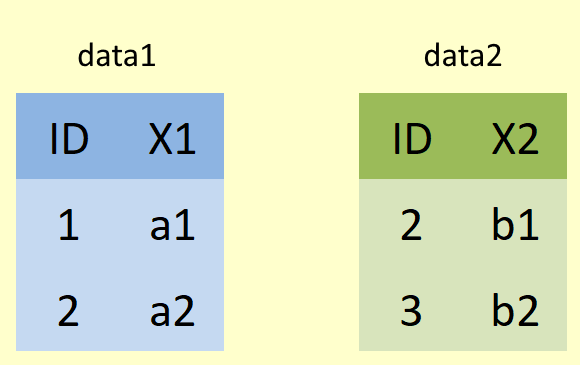
To make things nice and clear to see, lets simplify our data a litte.
Summer_Rain <- wos_seasonal_rain %>%
  select(year, sum)

Summer_Sun <- wos_seasonal_sun %>%
  select(year, sum)

Summer_Rain
## # A tibble: 154 x 2
## year sum
## <dbl> <dbl>
## 1 1862 426.
## 2 1863 299.
## 3 1864 255.
## 4 1865 274.
## 5 1866 345.
## 6 1867 340.
## 7 1868 295.
## 8 1869 183.
## 9 1870 205.
## 10 1871 349.
## # ... with 144 more rowsSummer_Sun## # A tibble: 102 x 2
## year sum
## <dbl> <dbl>
## 1 1919 524.
## 2 1920 411.
## 3 1921 509
## 4 1922 385.
## 5 1923 327.
## 6 1924 329.
## 7 1925 529.
## 8 1926 512.
## 9 1927 446
## 10 1928 408.
## # ... with 92 more rows
Now we have; * rain data for the summer months from 1862 to 2015 (Summer_Rain) * sunshine data for the summer months from 1919 to 2020 (Summer_Sun) Notice they have data from some of the same years, but also have data from years unique to each table
4.4.2.1 inner_join()
inner_join() returns all rows from both tables for which the values in column specified in the "by = " statement overlap.
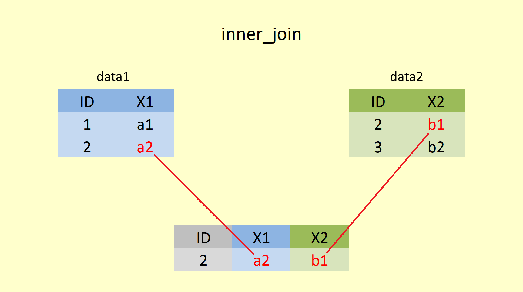
Here we merge Summer_Sun and Summer_Rain with inner_join() specifying we want to "join by" the variable year. Becuase the remaining variable has the same name in both tables, R needs to distiguish them from each other, for that we use the suffix = arguement, which allows us to specify what suffix to add to each column of the resulting table. If we do not spcify this, R will add a .x and .y suffix for us to the x (left) and y (right) table variables respectively.
inner <- inner_join(Summer_Sun, Summer_Rain, by="year", suffix = c("_sun", "_rain"))
inner
## # A tibble: 97 x 3
## year sum_sun sum_rain
## <dbl> <dbl> <dbl>
## 1 1919 524. 298
## 2 1920 411. 358.
## 3 1921 509 354.
## 4 1922 385. 334.
## 5 1923 327. 444.
## 6 1924 329. 395.
## 7 1925 529. 228.
## 8 1926 512. 367
## 9 1927 446 433.
## 10 1928 408. 440.
## # ... with 87 more rowsUsing an inner join returns only 97 (1919 to 2015) rows of observations because these are the only years in year that are present in both the Sun (1919 to 2020) and the Rain (1862 to 2015) data tables. However, we are still merging both tibbles together, meaning that all columns from Summer_Sun and Summer_Rain are kept (in our case sum, with a suffix added to each to tell them appart). In this example, the years 1862 to 1918, are dropped becuase they are not present in the Sun data, and the years 2016 to 2020 are dropped becuase they are not present in the Rain data.
If you don't specify which variable to "join by", and omit the by statement, the R will joing by all columns in common...
Try it for yourself in the Console and see what happens
Question Time
How many rows (or observations) does inner have?
How many columns (or variables) does inner have?
4.4.2.2 left_join()
left_join() retains the complete first (left) table and adds values from the second (right) table that have matching values in the column specified in the "by =" statement. Rows in the left table with no match in the right table will have missing values (NA) in the new columns.
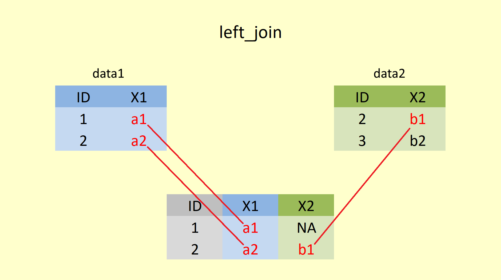
Let's try this left_join() function for our simple example of Summer_Sun and Summer_Rain in R.
left <- left_join(Summer_Sun, Summer_Rain, by="year", suffix = c("_sun", "_rain"))
left
## # A tibble: 102 x 3
## year sum_sun sum_rain
## <dbl> <dbl> <dbl>
## 1 1919 524. 298
## 2 1920 411. 358.
## 3 1921 509 354.
## 4 1922 385. 334.
## 5 1923 327. 444.
## 6 1924 329. 395.
## 7 1925 529. 228.
## 8 1926 512. 367
## 9 1927 446 433.
## 10 1928 408. 440.
## # ... with 92 more rowsHere Summer_Sun is returned in full, and for every matching year in Summer_Rain the value is added. However, Summer_Rain does not have any value for the years 2016 to 2020, hence NA is added here to the column sum_rain.
Question Time
How many rows (or observations) does left have?
How many columns (or variables) does left have?
4.4.2.3 right_join()
right_join() retains the complete second (right) table and adds values from the first (left) table that have matching values in the column specified in the by statement. Rows in the right table with no match in the left table will have missing values (NA) in the new columns.
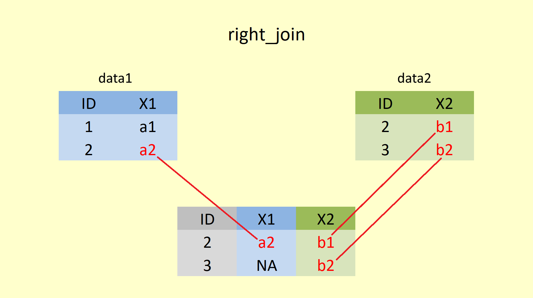
However, code-wise, you would still enter x as the first, and y as the second argument within right_join().
right <- right_join(Summer_Sun, Summer_Rain, by="year", suffix = c("_sun", "_rain"))
right
## # A tibble: 154 x 3
## year sum_sun sum_rain
## <dbl> <dbl> <dbl>
## 1 1919 524. 298
## 2 1920 411. 358.
## 3 1921 509 354.
## 4 1922 385. 334.
## 5 1923 327. 444.
## 6 1924 329. 395.
## 7 1925 529. 228.
## 8 1926 512. 367
## 9 1927 446 433.
## 10 1928 408. 440.
## # ... with 144 more rowsHere Summer_Rain is returned in full, and for every matching year in Summer_Sun the value is added, for any row of Summer_Rain that does not have a mating value in Summer_Sun, NA is added. Notice the order of the rows, though!!! All the years of Summer_Sun come first before the extra rows from Summer_Rain are added at the bottom. That is due to the order of how they are entered into the right_join() function. The "left" data (first table) is still prioritised in terms of ordering observations!
Question Time
How many rows (or observations) does right have?
4.4.2.4 full_join()
full_join() returns all rows and all columns from both dataframes. NA values fill unmatched rows.
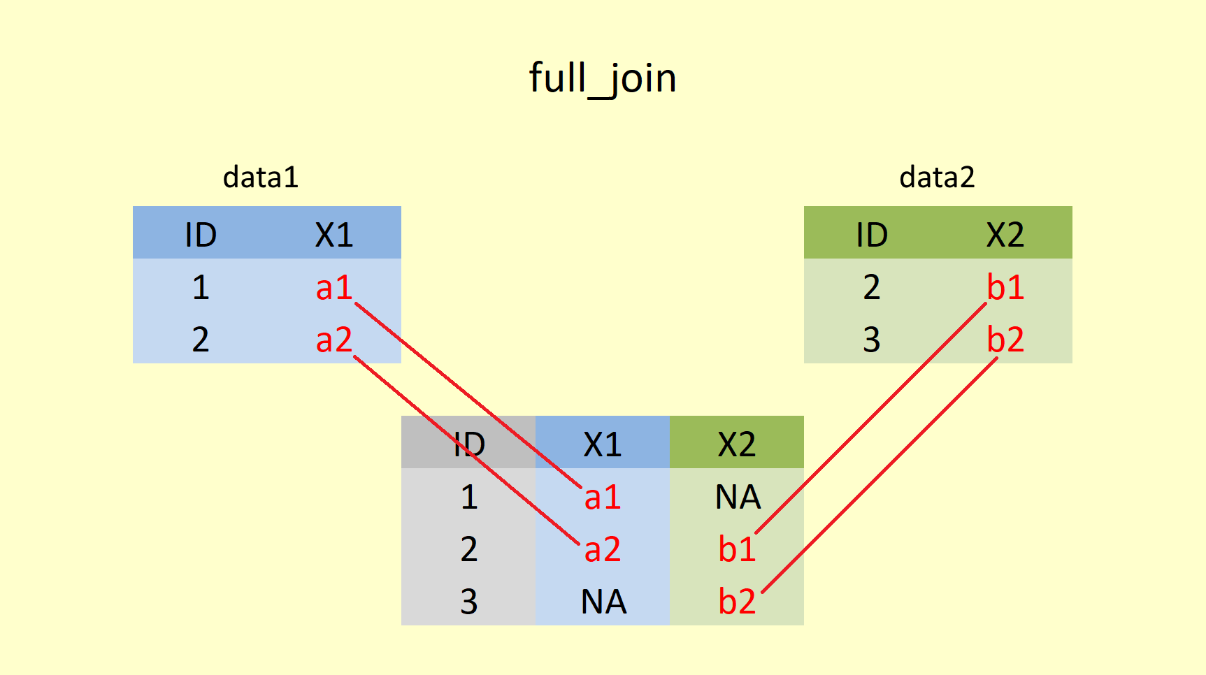
full <- full_join(Summer_Sun, Summer_Rain, by="year", suffix = c("_sun", "_rain"))
full
## # A tibble: 159 x 3
## year sum_sun sum_rain
## <dbl> <dbl> <dbl>
## 1 1919 524. 298
## 2 1920 411. 358.
## 3 1921 509 354.
## 4 1922 385. 334.
## 5 1923 327. 444.
## 6 1924 329. 395.
## 7 1925 529. 228.
## 8 1926 512. 367
## 9 1927 446 433.
## 10 1928 408. 440.
## # ... with 149 more rowsAs you can see, all years from both tables are kept, and NA is used to fill the missing years (1862 to 1918 for sum_sun, and 2016 to 2020 for sum_rain). Again you can see the prioritization of the left (first) table in the arrangement of the years.
Question Time
How many rows (or observations) does full have?
4.4.3 Mutating Join Summary
| join function | Description |
|---|---|
| inner_join() | Includes all rows that are PRESENT IN BOTH the left and the right table |
| left_join() | Includes all rows from the left table (first data entered) |
| left_join() | Includes all rows from the right table (second data entered) |
| full_join() | Includes all rows from both left and right tables |
Question Time
Your turn
Join together wos_seasonal_rain and wos_seasonal_sun so that we keep all the rows from the wos_seasonal_sun table, add a useful suffix so you can differentiate between columns with the same name. Store the result in Q10.
#Jaimie's solution
Q10 <- left_join(wos_seasonal_sun, wos_seasonal_rain, by = "year", suffix = c("_sun", "_rain"))
#OR
Q10 <- right_join(wos_seasonal_rain, wos_seasonal_sun, by = "year", suffix = c("_rain", "_sun"))

Q10
## # A tibble: 102 x 9
## year win_rain spr_rain sum_rain aut_rain win_sun spr_sun sum_sun aut_sun
## <dbl> <dbl> <dbl> <dbl> <dbl> <dbl> <dbl> <dbl> <dbl>
## 1 1919 389. 260. 298 339. NA 414. 524. 257.
## 2 1920 704. 428. 358. 374. 111. 328. 411. 219.
## 3 1921 489. 390. 354. 340. 104. 404. 509 222.
## 4 1922 620 309. 334. 290. 102. 457. 385. 252.
## 5 1923 531. 266. 444. 649. 77.2 430. 327. 245.
## 6 1924 406. 262. 395. 447. 117. 356 329. 221.
## 7 1925 575. 462. 228. 329. 87.5 353. 529. 252.
## 8 1926 547. 308. 367 547. 91.1 366. 512. 241.
## 9 1927 445. 345. 433. 574. 104. 423. 446 240.
## 10 1928 567. 272. 440. 612. 131. 384. 408. 253.
## # ... with 92 more rows4.4.4 Binding Join Verbs
In contrast to mutating join verbs, binding join verbs simply combine tables without any need for matching. Dplyr provides bind_rows() and bind_cols() for combining tables by row and column respectively. When row binding, missing columns are replaced by NA values. When column binding, if the tables do not match by appropriate dimensions, an error will result.
4.4.4.1 bind_rows()
bind_rows() is ideal when you have more entries of the same kind of data, i.e. new observations of the same variables. (For example; you have a new batch of participants answering the same questionnaire; or you have new air pollution data from a different geographic region... same variables - different observations)
Lets split some data
Sun_Season_1 <- wos_seasonal_sun %>%
  filter(year >= 1970)

Sun_Season_2 <- wos_seasonal_sun %>%
  filter(year < 1970)
Now we have 2 indetical tables for seasonal sunshine in the west of Scotland, but for different sets of years. All the same variables, but totally different observations.
We can easily join these together with bind_rows to create a complete history.
Bind_1 <- bind_rows(Sun_Season_1, Sun_Season_2)
Bind_1
## # A tibble: 102 x 5
## year win spr sum aut
## <dbl> <dbl> <dbl> <dbl> <dbl>
## 1 1970 158. 385. 474. 202.
## 2 1971 115. 424. 475. 269
## 3 1972 113. 380. 480. 282.
## 4 1973 116. 418. 444. 250
## 5 1974 110. 471. 480. 244
## 6 1975 130. 517. 561. 218.
## 7 1976 110. 343. 588. 213
## 8 1977 156. 431. 599. 226.
## 9 1978 159. 394. 412. 192.
## 10 1979 155. 383. 403. 223.
## # ... with 92 more rowsbind_rows() takes the second table Sun_Season_2 and puts it directly underneath the first table Sun_Season_1.
What happens if we attempt to bind tables with different dimensions
Bind_2 <- bind_rows(Sun_Season_1, inner)
Bind_2
## # A tibble: 148 x 7
## year win spr sum aut sum_sun sum_rain
## <dbl> <dbl> <dbl> <dbl> <dbl> <dbl> <dbl>
## 1 1970 158. 385. 474. 202. NA NA
## 2 1971 115. 424. 475. 269 NA NA
## 3 1972 113. 380. 480. 282. NA NA
## 4 1973 116. 418. 444. 250 NA NA
## 5 1974 110. 471. 480. 244 NA NA
## 6 1975 130. 517. 561. 218. NA NA
## 7 1976 110. 343. 588. 213 NA NA
## 8 1977 156. 431. 599. 226. NA NA
## 9 1978 159. 394. 412. 192. NA NA
## 10 1979 155. 383. 403. 223. NA NA
## # ... with 138 more rowsNotice that the bind_rows() does not "care" if it duplicates rows, here we have repeat years. Also bind_rows() does not "care" that there are columns that do not match between the tables, here NA is added fill the missing space.
4.4.4.2 bind_cols()
bind_cols() is similar to our mutating join verbs in that it creates a new table by joining columns (or variables) together. However, note that bind_cols() does not perform any kind of row-wise matching when joining tables.
Bind_3 <- bind_cols(wos_monthly_sun, wos_seasonal_sun)## New names:
## * year -> year...1
## * year -> year...15bind_cols()takes wos_seasonal_sun and puts it right next to wos_monthly_sun. Since the column name year is in both tables they get called year..1 and year...15 after their respective column number to differentiate them.
What happens if we attempt to bind tables with different dimensions
Bind_4 <- bind_cols(Summer_Sun, Summer_Rain)## Error: Can't recycle `..1` (size 102) to match `..2` (size 154).You simply get an error
By the way, you can merge as many data objects as you like with the binding functions, whereas in the join functions, you are limited to two. However, you could use a pipe to combine the merged dataframe with a third.
example 1: bind_rows(data1, data2, data3)
example 2: full_join(data1, data2) %>% full_join(data3)
Just to further clarify the differences between bind_cols() and the mutating joing verbs, lets look at how they would deal with the same challenge
First lets create a new table for winter sun data, but lets arrange it by "win", so that rather than being in order of year, it is in order of most sunshine. This will have the same dimensions as the Summer_Sun table but a totally different order
Winter_Sun <- wos_seasonal_sun %>%
  select(year, win) %>%
  arrange(desc(win))
Winter_Sun
## # A tibble: 102 x 2
## year win
## <dbl> <dbl>
## 1 1963 204.
## 2 2018 170.
## 3 2003 169.
## 4 2001 166
## 5 1965 165
## 6 2004 163.
## 7 1978 159.
## 8 1968 159.
## 9 1970 158.
## 10 1996 156.
## # ... with 92 more rowsNow lets try joining Winter_Sun and Summer_Sun using the two different methods
Comparison_1 <- bind_cols(Summer_Sun, Winter_Sun)## New names:
## * year -> year...1
## * year -> year...3Comparison_2 <- left_join(Summer_Sun, Winter_Sun, "year")
Comparison_1## # A tibble: 102 x 4
## year...1 sum year...3 win
## <dbl> <dbl> <dbl> <dbl>
## 1 1919 524. 1963 204.
## 2 1920 411. 2018 170.
## 3 1921 509 2003 169.
## 4 1922 385. 2001 166
## 5 1923 327. 1965 165
## 6 1924 329. 2004 163.
## 7 1925 529. 1978 159.
## 8 1926 512. 1968 159.
## 9 1927 446 1970 158.
## 10 1928 408. 1996 156.
## # ... with 92 more rowsComparison_2## # A tibble: 102 x 3
## year sum win
## <dbl> <dbl> <dbl>
## 1 1919 524. NA
## 2 1920 411. 111.
## 3 1921 509 104.
## 4 1922 385. 102.
## 5 1923 327. 77.2
## 6 1924 329. 117.
## 7 1925 529. 87.5
## 8 1926 512. 91.1
## 9 1927 446 104.
## 10 1928 408. 131.
## # ... with 92 more rowsUsing bind_cols() simply "copy and pasted" the two tables together, the fact that the rows were in different orders did not matter. On the other hand, using left_join() meant that R compared the content of "year" and matched them up, ignoring the fact that Winter_Sun was in a different arrangement.
4.5 Additional information
Garrick Aden-Buie created some amazing gganimation gif to illustrate how the joins work. Check it out! https://www.garrickadenbuie.com/project/tidyexplain/
4.6 Summative Homework
The second summative assignment is available on moodle now.
Good luck.
Check that your Rmd file knits into a html file before submitting. Upload your Rmd file (not the knitted html) to moodle.