Chapter 3 Data Transformation 1: Basic One Table Verbs

Intended Learning Outcomes

Be able to use the following dplyr one-table verbs:

• select()
• arrange()
• filter()
• mutate()
• group_by()
• summarise()

This lesson is led by Jaimie Torrance.

3.1 Data Wrangling

It is estimated that data scientists spend between 50-80% of their time cleaning and preparing data. This so-called data wrangling is a crucial first step in organising data for subsequent analysis (NYTimes., 2014). The goal is generally to get the data into a "tidy" format whereby each variable is a column, each observation is a row and each value is a cell. The tidyverse package, developed by Hadley Wickham, is a collection of R packages built around this basic concept and intended to make data science fast, easy and fun. It contains six core packages: dplyr, tidyr, readr, purrr, ggplot2, and tibble.

dplyr provides a useful selection of functions - each corresponding to a basic verb:

dplyr function	description
select()	Include or exclude certain variables (columns)
arrange()	Reorder observations (rows)
filter()	Include or exclude certain observations (rows)
mutate()	Create new variables (columns) and preserve existing ones
group_by()	Organise observations (rows) by variables (columns)
summarise()	Compute summary statistics for selected variables (columns)

These are termed one table verbs as they only operate on one table at a time. Today we will examine the Wickham Six; select(), arrange(), filter(), mutate(), group_by(), and summarise().

3.2 Pre-Steps

Before we can talk about today's data, let's do some house-keeping first.

3.2.1 Downloading materials

Download the materials we will be working with today from moodle. The zip folder that contains an Rmd file called L3_stub, and a data file called CareerStats.csv. Similar to last week, L3_stub contains all code chunks for today's lesson, and is intended for you to add notes and comments.

3.2.2 Unzipping the zip folder

Make sure you unzip the folder and check it contains the L3_stub.Rmd and CareerStats.csv.

3.2.3 Setting the working directory

Set that folder as your working directory for today. The files in the folders should now be visible in the Files pane.

3.2.4 Loading in the required packages into the library

As we will be using functions that are part of tidyverse, we need to load it into the library. You will also need to load in the new package babynames. You will need to have this package installed first before you can load it into the library, if you haven't done that yet use the install.packages() function down in your console first.

library(tidyverse)
library(babynames)

3.2.5 Read in the data

Now, today we will work with two different datasets, one fairly simple dataset, and another more messy complex dataset later one.

The first is a large dataset about babynames (big surprise!). The package you installed and loaded into the library is infact a readymade dataset, that can be read straight into the Global Environment. We will deal with the second dataset later.

Name_Data <- babynames

3.2.6 View the data

Click on Name_Data in your Global Environment to open your data in a new tab on the Source pane or call the object in your Console (by typing the name of the object Name_Data) to check that the data was correctly imported into R.

Name_Data

## # A tibble: 1,924,665 x 5
##     year sex   name          n   prop
##    <dbl> <chr> <chr>     <int>  <dbl>
##  1  1880 F     Mary       7065 0.0724
##  2  1880 F     Anna       2604 0.0267
##  3  1880 F     Emma       2003 0.0205
##  4  1880 F     Elizabeth  1939 0.0199
##  5  1880 F     Minnie     1746 0.0179
##  6  1880 F     Margaret   1578 0.0162
##  7  1880 F     Ida        1472 0.0151
##  8  1880 F     Alice      1414 0.0145
##  9  1880 F     Bertha     1320 0.0135
## 10  1880 F     Sarah      1288 0.0132
## # ... with 1,924,655 more rows

You could also view the data by using the function View(). If you are more of a typer than a mouse-user you can type View(Name_Data) into your Console. This will open the data in a read-only, spreadsheet-like format in a new tab on the Source pane.

Remember from last week, we can also use glimpse() to view the columns and their datatypes.

glimpse(Name_Data)

## Rows: 1,924,665
## Columns: 5
## $ year <dbl> 1880, 1880, 1880, 1880, 1880, 1880, 1880, 1880, 1880, 1880, 18...
## $ sex  <chr> "F", "F", "F", "F", "F", "F", "F", "F", "F", "F", "F", "F", "F...
## $ name <chr> "Mary", "Anna", "Emma", "Elizabeth", "Minnie", "Margaret", "Id...
## $ n    <int> 7065, 2604, 2003, 1939, 1746, 1578, 1472, 1414, 1320, 1288, 12...
## $ prop <dbl> 0.07238359, 0.02667896, 0.02052149, 0.01986579, 0.01788843, 0....

head() would be helpful in displaying only the first 6 rows of the dataset, but remember not to get "tricked" by the number of observations shown in the output.

head(Name_Data)

## # A tibble: 6 x 5
##    year sex   name          n   prop
##   <dbl> <chr> <chr>     <int>  <dbl>
## 1  1880 F     Mary       7065 0.0724
## 2  1880 F     Anna       2604 0.0267
## 3  1880 F     Emma       2003 0.0205
## 4  1880 F     Elizabeth  1939 0.0199
## 5  1880 F     Minnie     1746 0.0179
## 6  1880 F     Margaret   1578 0.0162

Question Time

How many rows (or observations) does Name_Data have?
How many columns (or variables) does Name_Data have?

Take some time to familiarise yourself with the variables in your dataframe.

3.3 select()

You may not want to include every single variable in your analysis. In order to include or exclude certain variables (columns), use the select() function. The first argument to this function is the object you want to select variables from (i.e. our tibble called Name_Data), and the subsequent arguments are the variables to keep.

For example, if you wanted to keep all variables except from prop, you could type:

select(Name_Data, year, sex, name, n)

## # A tibble: 1,924,665 x 4
##     year sex   name          n
##    <dbl> <chr> <chr>     <int>
##  1  1880 F     Mary       7065
##  2  1880 F     Anna       2604
##  3  1880 F     Emma       2003
##  4  1880 F     Elizabeth  1939
##  5  1880 F     Minnie     1746
##  6  1880 F     Margaret   1578
##  7  1880 F     Ida        1472
##  8  1880 F     Alice      1414
##  9  1880 F     Bertha     1320
## 10  1880 F     Sarah      1288
## # ... with 1,924,655 more rows

That works fine when you have realtively few variables like this dataset, however this menthod can become very time consuming if you have a lot of varibales in your dataset. There are two ways on how we could have done this easier and faster:

1. We could use the colon operator :. Similar to last week where we used the colon operator for numerical sequences, we can use it here for selecting a sequence of column names. Here, it reads as "take object student_HM, and select columns year, and every other column though to n".

select(Name_Data, year:n)

## # A tibble: 1,924,665 x 4
##     year sex   name          n
##    <dbl> <chr> <chr>     <int>
##  1  1880 F     Mary       7065
##  2  1880 F     Anna       2604
##  3  1880 F     Emma       2003
##  4  1880 F     Elizabeth  1939
##  5  1880 F     Minnie     1746
##  6  1880 F     Margaret   1578
##  7  1880 F     Ida        1472
##  8  1880 F     Alice      1414
##  9  1880 F     Bertha     1320
## 10  1880 F     Sarah      1288
## # ... with 1,924,655 more rows

2. We could use "negative selection", i.e. select the variable we wanted to drop by adding a minus in front of it.

select(Name_Data, -prop)

## # A tibble: 1,924,665 x 4
##     year sex   name          n
##    <dbl> <chr> <chr>     <int>
##  1  1880 F     Mary       7065
##  2  1880 F     Anna       2604
##  3  1880 F     Emma       2003
##  4  1880 F     Elizabeth  1939
##  5  1880 F     Minnie     1746
##  6  1880 F     Margaret   1578
##  7  1880 F     Ida        1472
##  8  1880 F     Alice      1414
##  9  1880 F     Bertha     1320
## 10  1880 F     Sarah      1288
## # ... with 1,924,655 more rows

We also have the option of "de-selecting" more than one variable. By including the minus sign before each column we can remove as many as we want.

select(Name_Data, -prop, -sex)

## # A tibble: 1,924,665 x 3
##     year name          n
##    <dbl> <chr>     <int>
##  1  1880 Mary       7065
##  2  1880 Anna       2604
##  3  1880 Emma       2003
##  4  1880 Elizabeth  1939
##  5  1880 Minnie     1746
##  6  1880 Margaret   1578
##  7  1880 Ida        1472
##  8  1880 Alice      1414
##  9  1880 Bertha     1320
## 10  1880 Sarah      1288
## # ... with 1,924,655 more rows

We can also use select() in combination with the c() function. Remember, c()is "hugging things together". We would put a single minus in front of the c rather than each of the column. This will read as exclude every column listed within the brackets.

select(Name_Data, -c(sex, n, prop))

Remember, if you don't save this data to an object (e.g. the original dataframe Name_Data or under a new name), it won't be saved. We have not saved any of the previous tasks to the Global Environment, so there should still be only one babynames related object, e.g. the tibble named Name_Data.

Question Time

Your turn

Create a tibble called Name_Short that keeps all variables/columns from the data Name_Data except from sex and n. Your new object Name_Short should appear in your Global Environment.

# Jaimie's solution:
Name_Short <- select(Name_Data, -sex, -n)
# OR
Name_Short <- select(Name_Data, -c(sex, n))
# OR
Name_Short <- select(Name_Data, year, name, prop)

You could also reference the position of column, rather than the actual name.

• select(Name_Data,1,3,5)

While it works code-wise, and seems a much quicker approach, it is a very bad idea in the name of reproducibility. If you send your code to a fellow researcher, they would have no idea what the code does. Moreover, if at some point, you need to add another column to your data, and/or decide to reorder the sequence of your columns, your code would not run anymore the way you expect it to.

3.4 arrange()

The arrange() function can reorder observations (rows) in ascending (default) or descending order. The first argument to this function is again an object (in this case the tibble Name_Data), and the subsequent arguments are the variables (columns) you want to sort by. For example, if you wanted to sort by n in ascending order (which is the default in arrange()) you would type:

Name_Arr <- arrange(Name_Data, n)
Name_Arr

## # A tibble: 1,924,665 x 5
##     year sex   name          n      prop
##    <dbl> <chr> <chr>     <int>     <dbl>
##  1  1880 F     Adelle        5 0.0000512
##  2  1880 F     Adina         5 0.0000512
##  3  1880 F     Adrienne      5 0.0000512
##  4  1880 F     Albertine     5 0.0000512
##  5  1880 F     Alys          5 0.0000512
##  6  1880 F     Ana           5 0.0000512
##  7  1880 F     Araminta      5 0.0000512
##  8  1880 F     Arthur        5 0.0000512
##  9  1880 F     Birtha        5 0.0000512
## 10  1880 F     Bulah         5 0.0000512
## # ... with 1,924,655 more rows

If you were to assign this code to the same object as before (i.e. Name_Data), the previous version of Name_Data would be overwritten.

Notice how the n column is now organised in alphabetical order i.e. smallest number to largest. Suppose you wanted to reverse this order, displaying largest, you would need to wrap the name of the variable in the desc() function (i.e. for descending).

Name_Arr2 <- arrange(Name_Data, desc(n))
Name_Arr2

## # A tibble: 1,924,665 x 5
##     year sex   name        n   prop
##    <dbl> <chr> <chr>   <int>  <dbl>
##  1  1947 F     Linda   99686 0.0548
##  2  1948 F     Linda   96209 0.0552
##  3  1947 M     James   94756 0.0510
##  4  1957 M     Michael 92695 0.0424
##  5  1947 M     Robert  91642 0.0493
##  6  1949 F     Linda   91016 0.0518
##  7  1956 M     Michael 90620 0.0423
##  8  1958 M     Michael 90520 0.0420
##  9  1948 M     James   88588 0.0497
## 10  1954 M     Michael 88514 0.0428
## # ... with 1,924,655 more rows

You can also sort by more than one column. For example, you could sort by name first, and then n second:

Name_Arr3 <- arrange(Name_Data, name, n)
Name_Arr3

## # A tibble: 1,924,665 x 5
##     year sex   name      n       prop
##    <dbl> <chr> <chr> <int>      <dbl>
##  1  2007 M     Aaban     5 0.00000226
##  2  2009 M     Aaban     6 0.00000283
##  3  2010 M     Aaban     9 0.00000439
##  4  2016 M     Aaban     9 0.00000446
##  5  2011 M     Aaban    11 0.00000542
##  6  2012 M     Aaban    11 0.00000543
##  7  2017 M     Aaban    11 0.0000056 
##  8  2013 M     Aaban    14 0.00000694
##  9  2015 M     Aaban    15 0.00000736
## 10  2014 M     Aaban    16 0.00000783
## # ... with 1,924,655 more rows

You can also arrange by multiple columns in desceding order too, or arrange by one column in ascending order and another in descending order if you wanted.

3.5 filter()

3.5.1 Single criterion

In order to include or exclude certain observations (rows), use the filter() function. The first argument to this function is an object (in this case the tibble Name_Data) and the subsequent argument is the criteria you wish to filter on. For example, if you want only those observations from the year of your birth:

Name_MyYear <- filter(Name_Data, year == 1988)
glimpse(Name_MyYear)

## Rows: 22,364
## Columns: 5
## $ year <dbl> 1988, 1988, 1988, 1988, 1988, 1988, 1988, 1988, 1988, 1988, 19...
## $ sex  <chr> "F", "F", "F", "F", "F", "F", "F", "F", "F", "F", "F", "F", "F...
## $ name <chr> "Jessica", "Ashley", "Amanda", "Sarah", "Jennifer", "Brittany"...
## $ n    <int> 51538, 49961, 39455, 28366, 27887, 26815, 22836, 20699, 20310,...
## $ prop <dbl> 0.02680669, 0.02598643, 0.02052190, 0.01475413, 0.01450499, 0....

or keep observations of only popular names:

Name_Pop <- filter(Name_Data, prop >= 0.07)
glimpse(Name_Pop)

## Rows: 19
## Columns: 5
## $ year <dbl> 1880, 1880, 1880, 1881, 1881, 1882, 1882, 1882, 1883, 1883, 18...
## $ sex  <chr> "F", "M", "M", "M", "M", "F", "M", "M", "M", "M", "M", "M", "M...
## $ name <chr> "Mary", "John", "William", "John", "William", "Mary", "John", ...
## $ n    <int> 7065, 9655, 9532, 8769, 8524, 8148, 9557, 9298, 8894, 8387, 93...
## $ prop <dbl> 0.07238359, 0.08154561, 0.08050676, 0.08098299, 0.07872038, 0....

1. Notice how we saved the new data under a different object name (Name_MyYear). When using filter(), you should never replace/ overwrite your original data unless you know exactly what you are doing. What could be the consequences?

2. By the way, what do symbols such == and >= remind you of??? (hint: something we covered last week?)

Consequences: You could potentially lose some data. Nothing is ever completely lost though (unless you are overwriting the original .csv file) but it could result in more work for you to restore everything from the beginning. Especially when your data scripts are very long and analysis is complex (i.e. taking up a lot of computing power), that could easily turn into a nightmare.

Remember the relational operators that returned logical values of either TRUE or FALSE?

Relational operators (such as ==, !=, <, <=, >, and >=) compare two numerical expressions and return a Boolean variable: a variable whose value is either 0 (FALSE) or 1 (TRUE). So, essentially, filter() includes any observations (rows) for which the expression evaluates to TRUE, and excludes any for which it evaluates to FALSE. In the previous example, filter() sifted through 1924665 observations, keeping rows containing year that was equal to 1998.

This works as well for columns of the data type character. If you want only those observations for a specific name, you could use the equivalence operator ==. Be aware that a single equals sign (=) is used to assign a value to a variable whereas a double equals sign (==) is used to check whether two values are equal.

Name_Me <- filter(Name_Data, name == "Jaimie")
glimpse(Name_Me)

## Rows: 118
## Columns: 5
## $ year <dbl> 1946, 1948, 1951, 1952, 1953, 1954, 1955, 1956, 1957, 1958, 19...
## $ sex  <chr> "F", "F", "F", "F", "F", "F", "F", "F", "F", "F", "M", "F", "M...
## $ name <chr> "Jaimie", "Jaimie", "Jaimie", "Jaimie", "Jaimie", "Jaimie", "J...
## $ n    <int> 7, 5, 8, 8, 6, 8, 12, 16, 9, 28, 12, 30, 13, 19, 10, 20, 7, 23...
## $ prop <dbl> 4.340e-06, 2.870e-06, 4.330e-06, 4.210e-06, 3.110e-06, 4.020e-...

Here, the filter() function compares every single value in the column name of the data object Name_Data with the character string written on the right-hand side of the equation ("Jaimie").

You can also use filter() to keep data from multiple options of the same variable using the %in% operator. In this case we want to filter several different names:

Name_J <- filter(Name_Data, name %in% c("Jaimie", "Jamie", "Jaime", "James", "Jayme"))
glimpse(Name_J)

## Rows: 963
## Columns: 5
## $ year <dbl> 1880, 1880, 1881, 1881, 1882, 1882, 1883, 1883, 1884, 1884, 18...
## $ sex  <chr> "F", "M", "F", "M", "F", "M", "F", "M", "F", "F", "M", "F", "M...
## $ name <chr> "James", "James", "James", "James", "James", "James", "James",...
## $ n    <int> 22, 5927, 24, 5441, 18, 5892, 25, 5223, 33, 5, 5693, 26, 5175,...
## $ prop <dbl> 0.00022540, 0.05005912, 0.00024278, 0.05024843, 0.00015558, 0....

Because filter() evalutes variables against your criteria and keeps observations that are TRUE, in essence the function defaults to "filter-in" certain observations. You can however also use it to "filter-out" specific observations, by using the 'not equals' operator !=. Here filter() keeps every row in which the value DOES NOT read what you have specificed.

Using filter() to exclude certain observations.

Name_J_Short <- filter(Name_J, name !="James")
glimpse(Name_J_Short)

## Rows: 687
## Columns: 5
## $ year <dbl> 1884, 1887, 1888, 1890, 1891, 1892, 1893, 1894, 1895, 1896, 18...
## $ sex  <chr> "F", "F", "F", "F", "F", "F", "F", "F", "F", "F", "M", "F", "M...
## $ name <chr> "Jamie", "Jamie", "Jamie", "Jamie", "Jamie", "Jamie", "Jamie",...
## $ n    <int> 5, 5, 5, 12, 11, 10, 9, 9, 10, 8, 6, 9, 5, 11, 14, 20, 6, 20, ...
## $ prop <dbl> 3.634e-05, 3.217e-05, 2.639e-05, 5.951e-05, 5.596e-05, 4.446e-...

3.5.2 Multiple criteria

Often you will come across a situation where you will need to filter based on multiple criteria. For that you have the options of AND and OR. ANDis used if you had two criteria and only wanted data returned when both criteria are met. ORis used if you had two criteria and wanted data returned for either criterion.

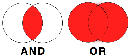
Simple Example: Just imagine, you have data of men and women who are either blond or dark-haired.

If you wanted to filter everyone who has blond hair AND is a man, all your data looks like this:

Whereas, if you wanted to filter out everyone who has either dark hair OR is a woman, you would get:

What does that mean for our babynames data?

For example, to filter rows containing only your name, of one sex, since your year of birth, you would code:

Name_Specific <- filter(Name_Data, name == "Jaimie", year >= 1988, sex == "M")
glimpse(Name_Specific)

## Rows: 19
## Columns: 5
## $ year <dbl> 1988, 1989, 1990, 1991, 1992, 1993, 1994, 1995, 1996, 1997, 19...
## $ sex  <chr> "M", "M", "M", "M", "M", "M", "M", "M", "M", "M", "M", "M", "M...
## $ name <chr> "Jaimie", "Jaimie", "Jaimie", "Jaimie", "Jaimie", "Jaimie", "J...
## $ n    <int> 22, 15, 28, 21, 19, 14, 6, 9, 10, 10, 6, 11, 9, 12, 7, 6, 6, 5, 5
## $ prop <dbl> 1.099e-05, 7.160e-06, 1.302e-05, 9.910e-06, 9.050e-06, 6.780e-...

You could have also used the logical operator & (AND) instead of the comma. filter(Name_Data, name == "Jaimie" & year >= 1988 & sex == "M") would have given you the same result as above.

If we wanted to filter the data Name_Data for either names with a very high count OR names that account for a very low proportion, we could use the logical operator | (OR).

Data_Or <- filter(Name_Data, n > 90000 | prop < 2.27e-06)
glimpse(Data_Or)

## Rows: 2,041
## Columns: 5
## $ year <dbl> 1947, 1947, 1947, 1948, 1949, 1956, 1957, 1958, 2007, 2007, 20...
## $ sex  <chr> "F", "M", "M", "F", "F", "M", "M", "M", "M", "M", "M", "M", "M...
## $ name <chr> "Linda", "James", "Robert", "Linda", "Linda", "Michael", "Mich...
## $ n    <int> 99686, 94756, 91642, 96209, 91016, 90620, 92695, 90520, 5, 5, ...
## $ prop <dbl> 0.05483812, 0.05101589, 0.04933934, 0.05521079, 0.05184643, 0....

As you will have noticed, Data_Or has now observations for names that either have a count over 90,000 in a year, or account for a very small proportion in a year. In this instance these are very distinct groups, and no observation would meet both criteria, check for yourself:

Data_Or2 <- filter(Name_Data, n > 90000 & prop < 2.27e-06)
glimpse(Data_Or2)

## Rows: 0
## Columns: 5
## $ year <dbl> 
## $ sex  <chr> 
## $ name <chr> 
## $ n    <int> 
## $ prop <dbl>

Here we see Data_Or2, returns no observations. However sometimes, you might select multiple criteria, where some observations will only meet one, but other observations may meet both criteria (see below). So always keep in mind what exactly you want to find, and choose the best way to filter.

Data_Or3 <- filter(Name_Data, n > 90000 | prop > 0.05)
glimpse(Data_Or3)

## Rows: 172
## Columns: 5
## $ year <dbl> 1880, 1880, 1880, 1880, 1881, 1881, 1881, 1881, 1882, 1882, 18...
## $ sex  <chr> "F", "M", "M", "M", "F", "M", "M", "M", "F", "M", "M", "F", "M...
## $ name <chr> "Mary", "John", "William", "James", "Mary", "John", "William",...
## $ n    <int> 7065, 9655, 9532, 5927, 6919, 8769, 8524, 5441, 8148, 9557, 92...
## $ prop <dbl> 0.07238359, 0.08154561, 0.08050676, 0.05005912, 0.06999140, 0....

Data_Or4 <- filter(Name_Data, n > 90000 & prop > 0.05)
glimpse(Data_Or4)

## Rows: 4
## Columns: 5
## $ year <dbl> 1947, 1947, 1948, 1949
## $ sex  <chr> "F", "M", "F", "F"
## $ name <chr> "Linda", "James", "Linda", "Linda"
## $ n    <int> 99686, 94756, 96209, 91016
## $ prop <dbl> 0.05483812, 0.05101589, 0.05521079, 0.05184643

Question Time

How many rows (or observations) does the object Data_Or3 contain?
How many different female names are in Data_Or4?

Your turn

Make a tibble called Name_Beat that only shows data from Name_Data for the names John, Paul, George and Ringo, and just for sex males.

Name_Beat <- filter(Name_Data, name %in% c("John", "Paul", "George", "Ringo"), sex == "M")

# If you have done this correct you should be able to produce a nice simple plot with the code below, to show change in proportional representation of these names over time (don't worry about what this code means, you'll learn more about plots later in the course)

ggplot(Name_Beat, aes(year, prop, colour=name)) + geom_line()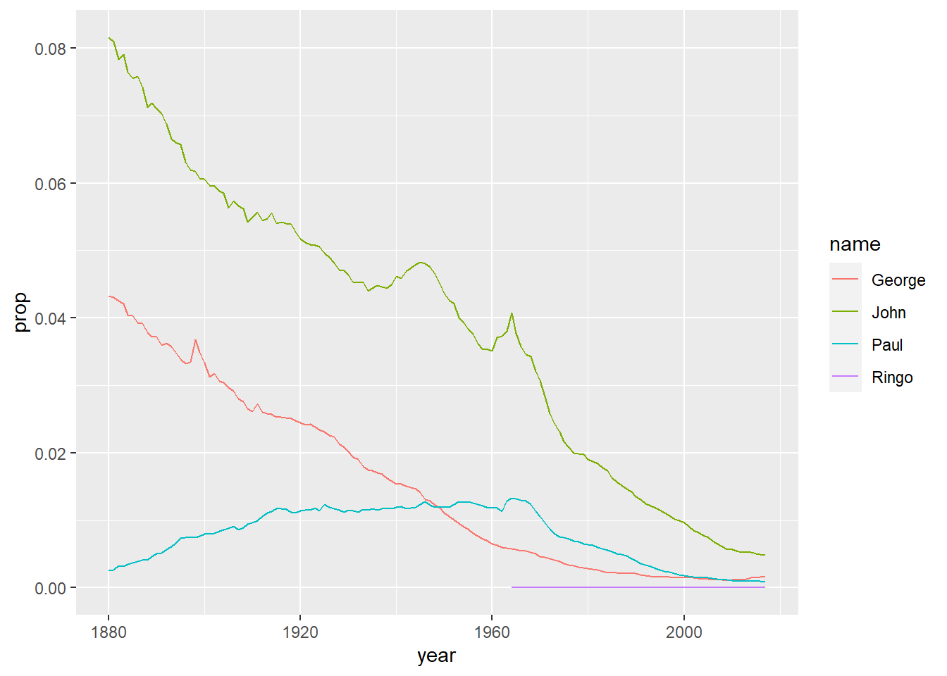

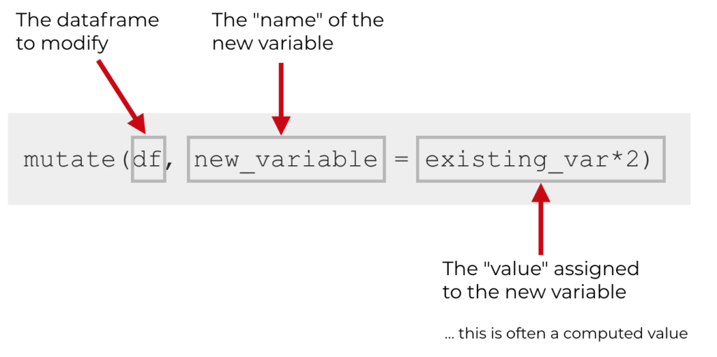
3.6 mutate()

The mutate() function creates new variables (columns) onto the existing object. The first argument to this function is an object from your Global Environment (for example Name_Data) and the subsequent argument is the new column name and what you want it to contain. The following image was downloaded from https://www.sharpsightlabs.com/blog/mutate-in-r/

Let's apply this to this to our Name_Data data tibble. Say we wanted to create a new column Decade that shows us the relative decade each observation is taken from. Save this as a new object Name_Ext to the Global Environment rather than overwriting Name_Data so that we can compare Name_Data with the extended Name_Ext later on.

Name_Ext <- mutate(Name_Data, Decade = floor(year/10)*10)
glimpse(Name_Ext)

## Rows: 1,924,665
## Columns: 6
## $ year   <dbl> 1880, 1880, 1880, 1880, 1880, 1880, 1880, 1880, 1880, 1880, ...
## $ sex    <chr> "F", "F", "F", "F", "F", "F", "F", "F", "F", "F", "F", "F", ...
## $ name   <chr> "Mary", "Anna", "Emma", "Elizabeth", "Minnie", "Margaret", "...
## $ n      <int> 7065, 2604, 2003, 1939, 1746, 1578, 1472, 1414, 1320, 1288, ...
## $ prop   <dbl> 0.07238359, 0.02667896, 0.02052149, 0.01986579, 0.01788843, ...
## $ Decade <dbl> 1880, 1880, 1880, 1880, 1880, 1880, 1880, 1880, 1880, 1880, ...

As we can see, Name_Ext has one column more than Name_Data. So mutate() took the value in the cells for each row of the variable year, devided it by 10, and using the floor() function, rounds that value down to the nearest whole number, before finally multiplying the result by 10, and adding it to a new column called Decade.

Importantly, new variables will overwrite existing variables if column headings are identical. So if we wanted to halve the values in column Decade and store them in a column Decade, the original Decade would be overwritten. To demonstrate we will try doing this and stroring the output in a new object called Name_Ext2and save that to our Global Environment.

Name_Ext2 <- mutate(Name_Ext, Decade = Decade/2)
glimpse(Name_Ext2)

## Rows: 1,924,665
## Columns: 6
## $ year   <dbl> 1880, 1880, 1880, 1880, 1880, 1880, 1880, 1880, 1880, 1880, ...
## $ sex    <chr> "F", "F", "F", "F", "F", "F", "F", "F", "F", "F", "F", "F", ...
## $ name   <chr> "Mary", "Anna", "Emma", "Elizabeth", "Minnie", "Margaret", "...
## $ n      <int> 7065, 2604, 2003, 1939, 1746, 1578, 1472, 1414, 1320, 1288, ...
## $ prop   <dbl> 0.07238359, 0.02667896, 0.02052149, 0.01986579, 0.01788843, ...
## $ Decade <dbl> 940, 940, 940, 940, 940, 940, 940, 940, 940, 940, 940, 940, ...

So now, Name_Ext2 did not gain a column (it still contains 6 variables), and Decade now has (unhelpfully) half the numeric value of the decade. (As an aside you could prevent yourself from accidentally doing something like this by converting Decade from numeric double type data to character type data, if you had no intention of carrying out any calculations on that variable)

The main take-away message here is to always check your data after manipulation if the outcome is really what you would expected. If you don't inspect and accidentally overwrite columns, you would not notice any difference.

You can also use mutate() to drop columns you no longer need, as an alternative to the select() function. This would mean that Name_Ext2 is now identical to Name_Data.

Name_Ext2 <- mutate(Name_Ext2, Decade = NULL)
glimpse(Name_Ext2)

## Rows: 1,924,665
## Columns: 5
## $ year <dbl> 1880, 1880, 1880, 1880, 1880, 1880, 1880, 1880, 1880, 1880, 18...
## $ sex  <chr> "F", "F", "F", "F", "F", "F", "F", "F", "F", "F", "F", "F", "F...
## $ name <chr> "Mary", "Anna", "Emma", "Elizabeth", "Minnie", "Margaret", "Id...
## $ n    <int> 7065, 2604, 2003, 1939, 1746, 1578, 1472, 1414, 1320, 1288, 12...
## $ prop <dbl> 0.07238359, 0.02667896, 0.02052149, 0.01986579, 0.01788843, 0....

If you want to add more than 2 columns, you can do that in a single mutate() statement. You can also add variables that are not numerical values, such as character or logical.

Add two columns to Name_Ext and call it Name_Ext3.

• Column 1 is called MinName and is of datatype logical. It contains a comparison of the value in n with the cut off count of 5 that allows inclusion in the dataset. Values of 5 should read TRUE, all other values FALSE.
• Column 2 is called "20thCent" and is of datatype logical. It contains a comparison of the value in years ensuring the value is between 1900 and 1999. Values inside this range should read TRUE, all other values FALSE.

Name_Ext3 <- mutate(Name_Ext, MinName = n == 5, "20thCent" = year >= 1900 & year <= 1999)
glimpse(Name_Ext3)

## Rows: 1,924,665
## Columns: 8
## $ year       <dbl> 1880, 1880, 1880, 1880, 1880, 1880, 1880, 1880, 1880, 18...
## $ sex        <chr> "F", "F", "F", "F", "F", "F", "F", "F", "F", "F", "F", "...
## $ name       <chr> "Mary", "Anna", "Emma", "Elizabeth", "Minnie", "Margaret...
## $ n          <int> 7065, 2604, 2003, 1939, 1746, 1578, 1472, 1414, 1320, 12...
## $ prop       <dbl> 0.07238359, 0.02667896, 0.02052149, 0.01986579, 0.017888...
## $ Decade     <dbl> 1880, 1880, 1880, 1880, 1880, 1880, 1880, 1880, 1880, 18...
## $ MinName    <lgl> FALSE, FALSE, FALSE, FALSE, FALSE, FALSE, FALSE, FALSE, ...
## $ `20thCent` <lgl> FALSE, FALSE, FALSE, FALSE, FALSE, FALSE, FALSE, FALSE, ...

You may have noticed we needed to put the name of our new column "20thCent" inside quotation marks. This is because that name would begin with numeric values which R will interpret as numeric values to be evaluated as code by default, which will then break our code. By placeing the name within quotation marks this tells R to treat this as a standard character string instead. It is always best to avoid creating variables with names that start with a number for this reason, but if it is necessary this is how you can work around it.

Your turn

• Add a new column to Name_Ext3 that is called Prcnt that gives the percentage each name accounts for of total names that year. *Hint: prop is that same stat represented as a proportion.

Name_Ext4 <- mutate(Name_Ext3, Prcnt = prop * 100)
glimpse(Name_Ext4)

## Rows: 1,924,665
## Columns: 9
## $ year       <dbl> 1880, 1880, 1880, 1880, 1880, 1880, 1880, 1880, 1880, 18...
## $ sex        <chr> "F", "F", "F", "F", "F", "F", "F", "F", "F", "F", "F", "...
## $ name       <chr> "Mary", "Anna", "Emma", "Elizabeth", "Minnie", "Margaret...
## $ n          <int> 7065, 2604, 2003, 1939, 1746, 1578, 1472, 1414, 1320, 12...
## $ prop       <dbl> 0.07238359, 0.02667896, 0.02052149, 0.01986579, 0.017888...
## $ Decade     <dbl> 1880, 1880, 1880, 1880, 1880, 1880, 1880, 1880, 1880, 18...
## $ MinName    <lgl> FALSE, FALSE, FALSE, FALSE, FALSE, FALSE, FALSE, FALSE, ...
## $ `20thCent` <lgl> FALSE, FALSE, FALSE, FALSE, FALSE, FALSE, FALSE, FALSE, ...
## $ Prcnt      <dbl> 7.238359, 2.667896, 2.052149, 1.986579, 1.788843, 1.6167...

3.6.1 Read in second dataset

At this point we are reaching the end of the usefulness of the Babynames dataset (there is only so much you can do with 5 basic variables), and this is a good time to bring in the second dataset we mentioned.

The second dataset, is a set of career and performance statistics of MMA athletes. You need to read the file CareerStats.csv containing your data into your Global Environment using the function read_csv(). Remember to store your data in an appropriately named object (e.g. MMA_Data).

MMA_Data <- read_csv("CareerStats.csv")

## 
## -- Column specification --------------------------------------------------------
## cols(
##   .default = col_double(),
##   ID = col_character(),
##   HeightClass = col_character(),
##   ReachClass = col_character(),
##   Stance = col_character(),
##   WeightClass = col_character()
## )
## i Use `spec()` for the full column specifications.

As you can see this dataset has a lot more variables, which should make for more interesting ways of manipulating the data.

3.7 summarise()

In order to compute summary statistics such as mean, median and standard deviation, use the summarise() function. This function creates a new tibble of your desired summary statistics. The first argument to this function is the data you are interested in summarising; in this case the object MMA_Data, and the subsequent argument is the new column name and what mathematical operation you want it to contain. You can add as many summary statistics in one summarise() function as you want; just separate them by a comma.

You can use the help function to find out more about the kind of summary stats you can extract.

Some of the most useful however are: sum() - sum total n() - count of observations n_distinct() - count of distinct (unique) observations mean() - measure of central tendency; mean median() - measure of central tendency; median sd() - standard deviation IQR() - interquartile range min() - the maximum available value in observations max() - the minimum available value in observations

Lets start generating some summary stats. For example, say you want to work out the average number of total fights (T_Fights) among the athletes and accompanying standard deviation for the entire sample:

summarise(MMA_Data, Avg_Mean = mean(T_Fights), SD = sd(T_Fights))

## # A tibble: 1 x 2
##   Avg_Mean    SD
##      <dbl> <dbl>
## 1     23.0  9.80

Therefore, the average number of total fights for all the athletes in our sample is 22.98, with a standard deviation of 9.8.

Let's try another. what is the maximum and minimum hights for the entire sample?

summarise(MMA_Data, Minimum = min(Height), Maximum = max(Height))

## # A tibble: 1 x 2
##   Minimum Maximum
##     <dbl>   <dbl>
## 1      63      83

Or maybe we want to know how many different (distinct) weightclasses are there in our dataset?

How would we check that?

summarise(MMA_Data, WeightClasses = n_distinct(WeightClass))

## # A tibble: 1 x 1
##   WeightClasses
##           <int>
## 1             8

3.8 Adding group_by()

Now that's all well and good, but in research we are most often interested in drawing comparisons and analysing differences (Between different groups of people, between different treatment types, between different countries etc.).

This is where the group_by() function comes in handy. It can organise observations (rows) by variables (columns), thereby spliting the data up into subsets that can be analysed independently. The first argument to this function is the data you wish to organise, in this case MMA_Data and the subsequent argument is your chosen grouping variable you want to organise by (e.g. group by). Here we are grouping by weightclass, and saving this as a new object MMA_G_Weight;

MMA_G_Weight <- group_by(MMA_Data, WeightClass)

If you view the object MMA_G_Class, it will not look any different to the original dataset (MMA_Data). However, be aware that the underlying structure has changed. In fact, you could use glimpse() to double check this.

glimpse(MMA_G_Weight)

## Rows: 199
## Columns: 32
## Groups: WeightClass [8]
## $ ID            <chr> "056c493bbd76a918", "b102c26727306ab6", "80eacd4da061...
## $ Age           <dbl> 31.88, 33.70, 34.41, 25.39, 31.02, 34.77, 33.97, 28.7...
## $ Height        <dbl> 64, 65, 64, 64, 65, 66, 64, 65, 65, 66, 67, 65, 68, 6...
## $ HeightClass   <chr> "Short", "Short", "Short", "Short", "Short", "Average...
## $ Weight        <dbl> 125, 125, 125, 125, 125, 125, 125, 125, 125, 125, 135...
## $ BMI           <dbl> 21.454, 20.799, 21.454, 21.454, 20.799, 20.173, 21.45...
## $ Reach         <dbl> 64, 67, 65, 63, 68, 66, 65, 67, 65, 65, 66, 65, 70, 6...
## $ ReachClass    <chr> "Below", "Below", "Below", "Below", "Below", "Below",...
## $ Stance        <chr> "Orthodox", "Orthodox", "Southpaw", "Orthodox", "Orth...
## $ WeightClass   <chr> "Flywieght", "Flywieght", "Flywieght", "Flywieght", "...
## $ T_Wins        <dbl> 13, 22, 26, 11, 15, 19, 23, 20, 19, 21, 15, 14, 12, 1...
## $ T_Losses      <dbl> 2, 5, 5, 3, 0, 7, 9, 3, 7, 5, 8, 1, 1, 5, 5, 4, 5, 2,...
## $ T_Fights      <dbl> 15, 27, 31, 14, 15, 26, 32, 23, 26, 26, 24, 15, 13, 1...
## $ Success       <dbl> 0.867, 0.815, 0.839, 0.786, 1.000, 0.731, 0.719, 0.87...
## $ W_by_Decision <dbl> 8, 12, 10, 4, 2, 8, 13, 6, 7, 11, 6, 7, 7, 1, 5, 3, 3...
## $ `W_by_KO/TKO` <dbl> 5, 10, 7, 1, 8, 8, 0, 6, 8, 4, 3, 2, 2, 8, 2, 2, 1, 4...
## $ W_by_Sub      <dbl> 0, 0, 9, 6, 5, 3, 10, 8, 4, 6, 6, 5, 3, 1, 5, 6, 10, ...
## $ L_by_Decision <dbl> 1, 3, 4, 2, 0, 4, 5, 3, 6, 1, 4, 0, 1, 3, 5, 1, 5, 0,...
## $ `L_by_KO/TKO` <dbl> 1, 2, 1, 0, 0, 2, 3, 0, 0, 1, 1, 1, 0, 0, 0, 2, 0, 2,...
## $ L_by_Sub      <dbl> 0, 0, 0, 1, 0, 1, 1, 0, 1, 3, 3, 0, 0, 2, 0, 1, 0, 0,...
## $ PWDec         <dbl> 0.533, 0.444, 0.323, 0.286, 0.133, 0.308, 0.406, 0.26...
## $ PWTko         <dbl> 0.333, 0.370, 0.226, 0.071, 0.533, 0.308, 0.000, 0.26...
## $ PWSub         <dbl> 0.000, 0.000, 0.290, 0.429, 0.333, 0.115, 0.312, 0.34...
## $ PLDec         <dbl> 0.067, 0.111, 0.129, 0.143, 0.000, 0.154, 0.156, 0.13...
## $ PLTko         <dbl> 0.067, 0.074, 0.032, 0.000, 0.000, 0.077, 0.094, 0.00...
## $ PLSub         <dbl> 0.000, 0.000, 0.000, 0.071, 0.000, 0.038, 0.031, 0.00...
## $ Available     <dbl> 9, 12, 24, 8, 4, 14, 12, 5, 15, 4, 10, 2, 1, 6, 5, 4,...
## $ TTime         <dbl> 123.234, 137.034, 278.699, 113.466, 42.700, 168.316, ...
## $ Time_Avg      <dbl> 13.693, 11.419, 11.612, 14.183, 10.675, 12.023, 12.12...
## $ TLpM          <dbl> 5.461, 3.196, 4.410, 2.732, 3.115, 3.624, 3.828, 5.85...
## $ AbpM          <dbl> 2.605, 2.167, 2.515, 1.921, 1.616, 2.549, 2.948, 3.37...
## $ SubAtt_Avg    <dbl> 0.122, 0.657, 0.700, 1.454, 3.864, 1.069, 0.618, 1.75...

You can now feed this grouped dataset (MMA_G_Weight) into the previous code line to obtain summary statistics by WeightClass, the code for finding summary statistics of average number of total fights, has been provided.:

Sum_Fights <- summarise(MMA_G_Weight, Avg_Mean = mean(T_Fights), SD = sd(T_Fights))

## `summarise()` ungrouping output (override with `.groups` argument)

Question Time

Which weightclass has the highest maximum height?

Your turn

• Try to fill out the code for finding summary stats of minimum and maximum height by WeightClass:

Sum_Height <- summarise(MMA_G_Weight, Minimum = min(Height), Maximum = max(Height))

## `summarise()` ungrouping output (override with `.groups` argument)

You can technically group by any variable! For example, there is nothing stopping you from grouping by a continuous variable like age or height. R will allow you to group by a numerical variable that is type double, the code will run.

However you probably want to be more careful in choosing a categorical variable as grouping criteria. These will usually be character, or interger or even logical data types. However interger data type might also actually represent a continuous variable (but might have only been recorded in whole numbers), and a variable that is character type may not represent a useful category (like idividual ID's for example).

The point is R does not know what your dataset is actually about, and what your variables are meant to represent... R has no idea if your variable should be categorical or not. So it's up to you to know what are sensible variables to use in the group_by() function.

You might also want to calculate and display the number of individuals from your dataset that are in different groups. This can be achieved by adding the summary function n() once you have grouped your data. the function n(), simply counts the number of observations and takes no arguments. Here we will group by Stance and count the number of athelets in each category:

MMA_G_Stance <- group_by(MMA_Data, Stance)

Stance_Ns <- summarise(MMA_G_Stance, N = n())

## `summarise()` ungrouping output (override with `.groups` argument)

Stance_Ns

## # A tibble: 3 x 2
##   Stance       N
##   <chr>    <int>
## 1 Orthodox   140
## 2 Southpaw    45
## 3 Switch      14

Question Time

How many athletes in the dataset have a Southpaw stance?
How many athletes in the dataset have an Orthodox stance?

Finally, it is possible to add multiple grouping variables. For example, the following code groups MMA_Data by ReachClass and Stance and then calculates the mean and standard deviation of average number of strikes landed per minute (TLpM) for each group (6 groups).

MMA_G_RS <- group_by(MMA_Data, ReachClass, Stance)
MMA_LpM <- summarise(MMA_G_RS, Mean = mean(TLpM), SD = sd(TLpM))

## `summarise()` regrouping output by 'ReachClass' (override with `.groups` argument)

MMA_LpM

## # A tibble: 6 x 4
## # Groups:   ReachClass [2]
##   ReachClass Stance    Mean    SD
##   <chr>      <chr>    <dbl> <dbl>
## 1 Above      Orthodox  5.44  1.66
## 2 Above      Southpaw  4.68  1.16
## 3 Above      Switch    5.92  1.29
## 4 Below      Orthodox  5.33  1.60
## 5 Below      Southpaw  5.02  1.47
## 6 Below      Switch    5.95  3.63

So far we have not had to calculate any summary statistics with any missing values, denoted by NA in R. Missing values are always a bit of a hassle to deal with. Any computation you do that involves NA returns an NA - which translates as "you will not get a numeric result when your column contains missing values". Missing values can be removed by adding the argument na.rm = TRUE to calculation functions like mean(), median() or sd(). For example, lets try to calulate a mean where we have some missing values:

Weight_Reach <- summarise(MMA_G_Weight, Avg_Reach = mean(Reach))

## `summarise()` ungrouping output (override with `.groups` argument)

Weight_Reach

## # A tibble: 8 x 2
##   WeightClass      Avg_Reach
##   <chr>                <dbl>
## 1 Bantamweight          67.8
## 2 Fetherweight          71.0
## 3 Flywieght             66.9
## 4 Heavyweight           NA  
## 5 LightHeavyweight      76.9
## 6 Lightweight           72.6
## 7 Middleweight          NA  
## 8 Welterweight          74

The code runs without error, however you will notice we have a few stats missing (NA). Now lets tell R to remove any missing values when making its calculation.

Weight_Reach <- summarise(MMA_G_Weight, Avg_Reach = mean(Reach, na.rm = T))

## `summarise()` ungrouping output (override with `.groups` argument)

Weight_Reach

## # A tibble: 8 x 2
##   WeightClass      Avg_Reach
##   <chr>                <dbl>
## 1 Bantamweight          67.8
## 2 Fetherweight          71.0
## 3 Flywieght             66.9
## 4 Heavyweight           78.0
## 5 LightHeavyweight      76.9
## 6 Lightweight           72.6
## 7 Middleweight          75.4
## 8 Welterweight          74

Finally... If you need to return the data to a non-grouped form, use the ungroup() function.

MMA_Data <- group_by(MMA_Data, BMI)
glimpse(MMA_Data)

## Rows: 199
## Columns: 32
## Groups: BMI [70]
## $ ID            <chr> "056c493bbd76a918", "b102c26727306ab6", "80eacd4da061...
## $ Age           <dbl> 31.88, 33.70, 34.41, 25.39, 31.02, 34.77, 33.97, 28.7...
## $ Height        <dbl> 64, 65, 64, 64, 65, 66, 64, 65, 65, 66, 67, 65, 68, 6...
## $ HeightClass   <chr> "Short", "Short", "Short", "Short", "Short", "Average...
## $ Weight        <dbl> 125, 125, 125, 125, 125, 125, 125, 125, 125, 125, 135...
## $ BMI           <dbl> 21.454, 20.799, 21.454, 21.454, 20.799, 20.173, 21.45...
## $ Reach         <dbl> 64, 67, 65, 63, 68, 66, 65, 67, 65, 65, 66, 65, 70, 6...
## $ ReachClass    <chr> "Below", "Below", "Below", "Below", "Below", "Below",...
## $ Stance        <chr> "Orthodox", "Orthodox", "Southpaw", "Orthodox", "Orth...
## $ WeightClass   <chr> "Flywieght", "Flywieght", "Flywieght", "Flywieght", "...
## $ T_Wins        <dbl> 13, 22, 26, 11, 15, 19, 23, 20, 19, 21, 15, 14, 12, 1...
## $ T_Losses      <dbl> 2, 5, 5, 3, 0, 7, 9, 3, 7, 5, 8, 1, 1, 5, 5, 4, 5, 2,...
## $ T_Fights      <dbl> 15, 27, 31, 14, 15, 26, 32, 23, 26, 26, 24, 15, 13, 1...
## $ Success       <dbl> 0.867, 0.815, 0.839, 0.786, 1.000, 0.731, 0.719, 0.87...
## $ W_by_Decision <dbl> 8, 12, 10, 4, 2, 8, 13, 6, 7, 11, 6, 7, 7, 1, 5, 3, 3...
## $ `W_by_KO/TKO` <dbl> 5, 10, 7, 1, 8, 8, 0, 6, 8, 4, 3, 2, 2, 8, 2, 2, 1, 4...
## $ W_by_Sub      <dbl> 0, 0, 9, 6, 5, 3, 10, 8, 4, 6, 6, 5, 3, 1, 5, 6, 10, ...
## $ L_by_Decision <dbl> 1, 3, 4, 2, 0, 4, 5, 3, 6, 1, 4, 0, 1, 3, 5, 1, 5, 0,...
## $ `L_by_KO/TKO` <dbl> 1, 2, 1, 0, 0, 2, 3, 0, 0, 1, 1, 1, 0, 0, 0, 2, 0, 2,...
## $ L_by_Sub      <dbl> 0, 0, 0, 1, 0, 1, 1, 0, 1, 3, 3, 0, 0, 2, 0, 1, 0, 0,...
## $ PWDec         <dbl> 0.533, 0.444, 0.323, 0.286, 0.133, 0.308, 0.406, 0.26...
## $ PWTko         <dbl> 0.333, 0.370, 0.226, 0.071, 0.533, 0.308, 0.000, 0.26...
## $ PWSub         <dbl> 0.000, 0.000, 0.290, 0.429, 0.333, 0.115, 0.312, 0.34...
## $ PLDec         <dbl> 0.067, 0.111, 0.129, 0.143, 0.000, 0.154, 0.156, 0.13...
## $ PLTko         <dbl> 0.067, 0.074, 0.032, 0.000, 0.000, 0.077, 0.094, 0.00...
## $ PLSub         <dbl> 0.000, 0.000, 0.000, 0.071, 0.000, 0.038, 0.031, 0.00...
## $ Available     <dbl> 9, 12, 24, 8, 4, 14, 12, 5, 15, 4, 10, 2, 1, 6, 5, 4,...
## $ TTime         <dbl> 123.234, 137.034, 278.699, 113.466, 42.700, 168.316, ...
## $ Time_Avg      <dbl> 13.693, 11.419, 11.612, 14.183, 10.675, 12.023, 12.12...
## $ TLpM          <dbl> 5.461, 3.196, 4.410, 2.732, 3.115, 3.624, 3.828, 5.85...
## $ AbpM          <dbl> 2.605, 2.167, 2.515, 1.921, 1.616, 2.549, 2.948, 3.37...
## $ SubAtt_Avg    <dbl> 0.122, 0.657, 0.700, 1.454, 3.864, 1.069, 0.618, 1.75...

MMA_Data <- ungroup(MMA_Data)
glimpse(MMA_Data)

## Rows: 199
## Columns: 32
## $ ID            <chr> "056c493bbd76a918", "b102c26727306ab6", "80eacd4da061...
## $ Age           <dbl> 31.88, 33.70, 34.41, 25.39, 31.02, 34.77, 33.97, 28.7...
## $ Height        <dbl> 64, 65, 64, 64, 65, 66, 64, 65, 65, 66, 67, 65, 68, 6...
## $ HeightClass   <chr> "Short", "Short", "Short", "Short", "Short", "Average...
## $ Weight        <dbl> 125, 125, 125, 125, 125, 125, 125, 125, 125, 125, 135...
## $ BMI           <dbl> 21.454, 20.799, 21.454, 21.454, 20.799, 20.173, 21.45...
## $ Reach         <dbl> 64, 67, 65, 63, 68, 66, 65, 67, 65, 65, 66, 65, 70, 6...
## $ ReachClass    <chr> "Below", "Below", "Below", "Below", "Below", "Below",...
## $ Stance        <chr> "Orthodox", "Orthodox", "Southpaw", "Orthodox", "Orth...
## $ WeightClass   <chr> "Flywieght", "Flywieght", "Flywieght", "Flywieght", "...
## $ T_Wins        <dbl> 13, 22, 26, 11, 15, 19, 23, 20, 19, 21, 15, 14, 12, 1...
## $ T_Losses      <dbl> 2, 5, 5, 3, 0, 7, 9, 3, 7, 5, 8, 1, 1, 5, 5, 4, 5, 2,...
## $ T_Fights      <dbl> 15, 27, 31, 14, 15, 26, 32, 23, 26, 26, 24, 15, 13, 1...
## $ Success       <dbl> 0.867, 0.815, 0.839, 0.786, 1.000, 0.731, 0.719, 0.87...
## $ W_by_Decision <dbl> 8, 12, 10, 4, 2, 8, 13, 6, 7, 11, 6, 7, 7, 1, 5, 3, 3...
## $ `W_by_KO/TKO` <dbl> 5, 10, 7, 1, 8, 8, 0, 6, 8, 4, 3, 2, 2, 8, 2, 2, 1, 4...
## $ W_by_Sub      <dbl> 0, 0, 9, 6, 5, 3, 10, 8, 4, 6, 6, 5, 3, 1, 5, 6, 10, ...
## $ L_by_Decision <dbl> 1, 3, 4, 2, 0, 4, 5, 3, 6, 1, 4, 0, 1, 3, 5, 1, 5, 0,...
## $ `L_by_KO/TKO` <dbl> 1, 2, 1, 0, 0, 2, 3, 0, 0, 1, 1, 1, 0, 0, 0, 2, 0, 2,...
## $ L_by_Sub      <dbl> 0, 0, 0, 1, 0, 1, 1, 0, 1, 3, 3, 0, 0, 2, 0, 1, 0, 0,...
## $ PWDec         <dbl> 0.533, 0.444, 0.323, 0.286, 0.133, 0.308, 0.406, 0.26...
## $ PWTko         <dbl> 0.333, 0.370, 0.226, 0.071, 0.533, 0.308, 0.000, 0.26...
## $ PWSub         <dbl> 0.000, 0.000, 0.290, 0.429, 0.333, 0.115, 0.312, 0.34...
## $ PLDec         <dbl> 0.067, 0.111, 0.129, 0.143, 0.000, 0.154, 0.156, 0.13...
## $ PLTko         <dbl> 0.067, 0.074, 0.032, 0.000, 0.000, 0.077, 0.094, 0.00...
## $ PLSub         <dbl> 0.000, 0.000, 0.000, 0.071, 0.000, 0.038, 0.031, 0.00...
## $ Available     <dbl> 9, 12, 24, 8, 4, 14, 12, 5, 15, 4, 10, 2, 1, 6, 5, 4,...
## $ TTime         <dbl> 123.234, 137.034, 278.699, 113.466, 42.700, 168.316, ...
## $ Time_Avg      <dbl> 13.693, 11.419, 11.612, 14.183, 10.675, 12.023, 12.12...
## $ TLpM          <dbl> 5.461, 3.196, 4.410, 2.732, 3.115, 3.624, 3.828, 5.85...
## $ AbpM          <dbl> 2.605, 2.167, 2.515, 1.921, 1.616, 2.549, 2.948, 3.37...
## $ SubAtt_Avg    <dbl> 0.122, 0.657, 0.700, 1.454, 3.864, 1.069, 0.618, 1.75...

3.9 Formative Homework

The folder for the formative assessment can now be downloaded from moodle.

1. Load tidyverse into the library.
2. Read the data from TraitJudgementData.csv into your Global Environment as an object called traits_data.
3. Look at the data. Familiarise yourself with the data (see next section, and the paper in the folder), as well as the datatypes of each column.

3.9.1 Brief introduction to the homework data

For the homework assignments each week, we will be using an open access dataset into how personality is determined from voices. A full version of the paper can be found https://journals.plos.org/plosone/article?id=10.1371/journal.pone.0204991. All data and sounds are available on OSF (osf.io/s3cxy).

However, for your assignment this week, all files necessary are compiled in a folder to download from moodle.

The data in the TraitJudgementData.csv has ratings on 3 different personality traits (Trustworthiness, Dominance, and Attractiveness) for 30 male and 30 female voice stimuli. In total, 181 participants rated either male OR female speakers on ONE personality trait (e.g. Trustworthiness) only. The speakers were judged after saying a socially relevant word ("Hello"), a socially ambiguous word ("Colors"), a socially relevant sentence ("I urge you to submit your essay by the end of the week"), and a socially ambiguous sentence ("Some have accepted it as a miracle without physical explanation"). Socially relevant stimuli were meant to address the listener, whereas socially ambiguous stimuli were intended to not be directed towards the listener. Each participant rated all the voice stimuli twice in all four conditions (socially relevant words (RW), socially relevant sentences (RS), socially ambiguous words (AW), and socially ambiguous sentences (AS)). The experiment was conducted online.

Here is a brief summary overview of the columns in the TraitJudgementData.csv.

column name	description
PP_ID	Participant's ID
PP_Age	Participant's Age
PP_Sex	Participant's Sex ("female", "male")
Nationality	Participant's Nationality
Trait	Personality Trait participant judged the vocal stimuli on ("Trustworthiness", "Dominance", "Attractiveness")
Voice	Speaker's ID
Voice_Sex	Speaker's Sex ("Female", "Male")
Condition	Speaker's recording of socially relevant words ("RW"), socially relevant sentences ("RS"), socially ambiguous words ("AW"), and socially ambiguous sentences ("AS")
Rating	Participants rated each Voice in each Condition twice ("Rating1", "Rating2")
Response	Participant's Trait judgements on a scale from 1 - 500
Reaction	Participant's Reaction Time